|
<< Click to Display Table of Contents >> Data Entry |
  
|
|
<< Click to Display Table of Contents >> Data Entry |
  
|
Open the Examples project and open Case 9.
General Tab

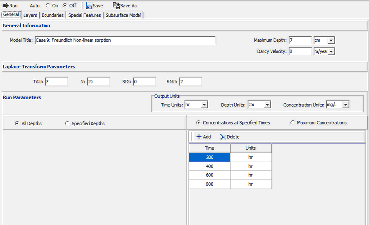
On the General tab the Darcy velocity is set to zero for pure diffusion. The concentrations can either be calculated at specified times or the time of the maximum concentration can be found. In this example the concentrations will be calculated at 4 times: 200, 400, 600, and 800 years.
Layers Tab

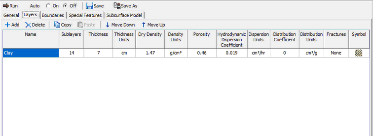
When using non-linear sorption the Distribution Coefficient is automatically calculated. The value entered on this tab is ignored by the program.There are no fractures in the layer. For pure diffusion even if there were fractures it should be modelled as if the soil was unfractured, since there would be no flow in the fractures for pure diffusion through the matrix.
Boundaries Tab

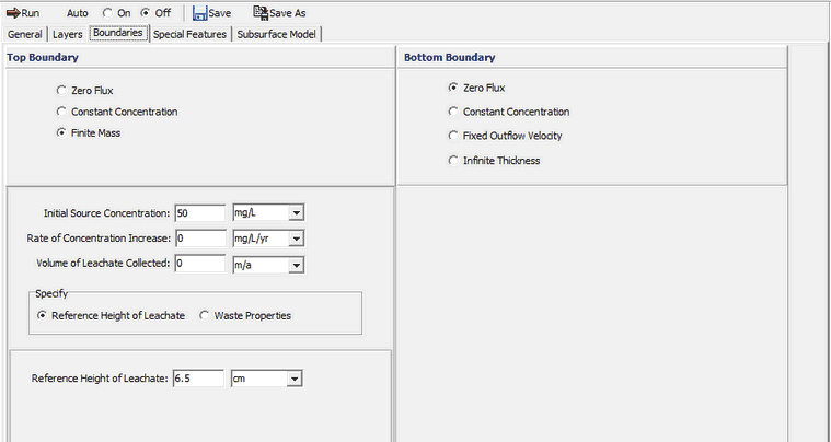
In this example, the top boundary has a finite mass and the bottom boundary is represented as a zero flux layer.
Special Features
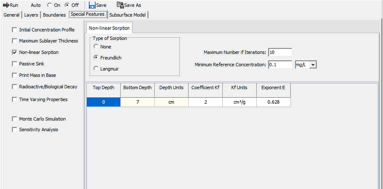
The non-linear sorption for this example is specified using the Special Features tab.
Non-linear Sorption

To specify the Freundlich non-linear sorption, check the Non-linear Sorption box on the Special Features tab. The Non-linear Sorption Data sub-tab can be used to specify the type of sorption as either Freundlich or Langmuir.
The Freundlich non-linear sorption parameters are determined experimentally. The iterative procedure used to determine the distribution coefficient is repeated until either the maximum change in concentrations between iterations is less than 0.1% or the
maximum number of iterations is reached. Minimum reference concentration is the minimum value that will be used in calculating the distribution coefficient. If the average concentration in a sub-layer is less than this minimum reference value, then the reference value is used in the calculation of the distribution coefficient.