

Sieve analysis calculations convert the masses retained on a series of sieves into a particle-size distribution. The basic arithmetic is simple: calculate cumulative retained mass, express it as a percentage of the appropriate total dry mass, and subtract that percentage from 100 to obtain percent passing. Reliable results still depend on specimen preparation, the applicable test method and mass checks.
This guide follows a synthetic 1,000 g example from retained masses to a grain-size curve. It focuses on understanding and checking the calculations rather than reproducing an entire laboratory procedure. Real soil and aggregate testing must use the method appropriate to the material, project and requested result.
Download the worked data
The learning examples pack contains sieve-analysis-example.csv with retained masses, cumulative masses and percentages. The worked-examples PDF provides a printable graph and calculation reference. The example closes exactly by design; it should not be mistaken for a measured specimen or a statement of allowable mass loss.
Establish the mass basis
Identify the total dry mass used in the calculation and how it was obtained. For the simplified example, that mass is 1,000 g. The masses retained on the successive sieves and in the pan sum to the same value. Real workflows may include washing, splitting, corrections or other preparation steps. Those operations affect how the result must be calculated and reconciled under the governing method.
Do not assume the sum of whatever appears in a spreadsheet is automatically the correct denominator. Compare it with the required original or adjusted specimen mass and document the relationship. A missing pan mass or omitted fraction can still produce a tidy column of percentages while misrepresenting the sample.
Work through the retained masses
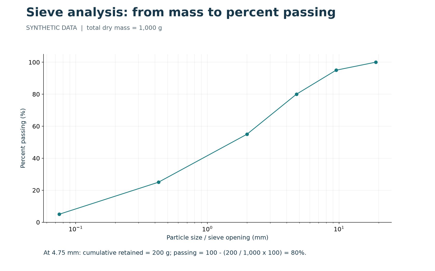
The example uses sieve openings of 19, 9.5, 4.75, 2.0, 0.425 and 0.075 mm, followed by a pan. Retained masses are respectively 0, 50, 150, 250, 300, 200 and 50 g. Cumulative retained mass is the running total from the largest opening down to the current sieve. At 4.75 mm, the cumulative mass is 0 + 50 + 150 = 200 g.
Percent retained on a single sieve is that sieve’s retained mass divided by the total dry mass, multiplied by 100. Cumulative percent retained uses the cumulative mass instead. The distinction matters: at 4.75 mm, the individual retained percentage is 15 percent, but the cumulative retained percentage is 20 percent. Using the individual figure to calculate passing would give the wrong answer.
Calculate percent passing
At 4.75 mm, cumulative percent retained is 200 / 1,000 x 100 = 20 percent. Percent passing is 100 – 20 = 80 percent. Repeating the calculation gives passing values of 100, 95, 80, 55, 25 and 5 percent at the six sieve openings. The final pan contains the material that passed the smallest listed sieve.
The pan is not a sieve with a zero-millimetre opening. Do not place it at zero on a logarithmic particle-size axis. Its mass contributes to the specimen balance and the interpretation of the finest measured fraction. Further characterization below the smallest sieve requires an appropriate additional method; the sieve calculation alone does not reveal the distribution within that fraction.
Plot the grain-size distribution
A typical grain-size distribution graph uses a logarithmic horizontal axis for particle size and a linear vertical axis for percent passing. Plot each measured opening against its passing percentage and label the units. The example figure displays larger particle sizes toward the right. If another report reverses the axis, read the scale carefully before comparing the visual slope.
Use enough measured points to represent the distribution, but avoid drawing a smooth-looking curve that implies unsupported detail. A sharp change may be meaningful or may indicate a problem requiring investigation. The graph should lead the reviewer back to the retained masses and preparation record, not conceal those records behind an attractive line.
Understand characteristic particle sizes
A characteristic size such as D10 represents the particle size at which ten percent passes, determined from the relevant curve within the supported measurement range. D30 and D60 are interpreted similarly. Where appropriate, these sizes can support gradation coefficients such as Cu = D60 / D10 and Cc = D30 squared / (D10 x D60).
When interpolation is justified on a semilogarithmic plot, treat the size axis logarithmically. Do not apply a simple arithmetic size average and assume it reproduces the graph. If a target passing percentage lies outside the measured range, do not invent a characteristic size to force a coefficient calculation. Review whether another test or a qualified interpretation is required.
Check the specimen balance and monotonicity
The retained masses should reconcile with the mass basis within the requirements of the procedure. Review discrepancies before normalizing everything to 100 percent. Normalization can hide a lost fraction, transcription error or incorrect specimen identifier. Keep any adjustment traceable and explain its basis in the laboratory record.
As sieve openings become smaller, cumulative retained mass should not decrease and percent passing should not increase. Negative masses, percentages outside zero to one hundred, duplicate openings or incorrectly sorted rows are useful warning signs. Investigate rather than merely sorting or clipping the results until the graph looks conventional.
Separate gradation from soil classification
Particle-size distribution contributes to soil classification, but it is not the whole classification process. Fines may require plasticity information, and the distinction between material fractions must use the applicable system. A specimen with a certain percent passing the No. 200 sieve should not be assigned a complete group symbol solely from that number.
For background, consult the FHWA soil-classification overview. For the soil sieve-analysis procedure, use the applicable edition of ASTM D6913/D6913M, identified in ASTM’s testing reference. Other materials and preparation operations may require different or additional methods. State what was actually performed.
Keep the report connected to the raw data
A useful report identifies the project, specimen, method, preparation, units and resulting distribution. Preserve retained masses and calculation records even when the client receives only a graph. If a sample name or mass changes, review the affected percentages, derived sizes and classification together. A revised PDF without a corresponding source correction creates an unreliable record for the next person.
The CSV supplied with this guide is a learning worksheet, not a guaranteed import format for every application. Map and validate fields before bringing external tables into production software. Check at least the specimen identity, openings, mass units, total mass and selected calculated points after transfer.
Continue with the GDMS workflow
GAEA’s sieve-analysis tutorial explains how to work with supported records and reporting in GDMS. Compare the example calculation with the software output as a learning exercise, then validate your actual laboratory method, settings and templates using approved specimens and procedures.
The strongest workflow makes the complete chain visible: source specimen, measured masses, checked calculation, graph and reviewed report. Automation can reduce repetitive arithmetic and formatting, while careful data management and technical review preserve confidence in what the curve represents.