
Overview
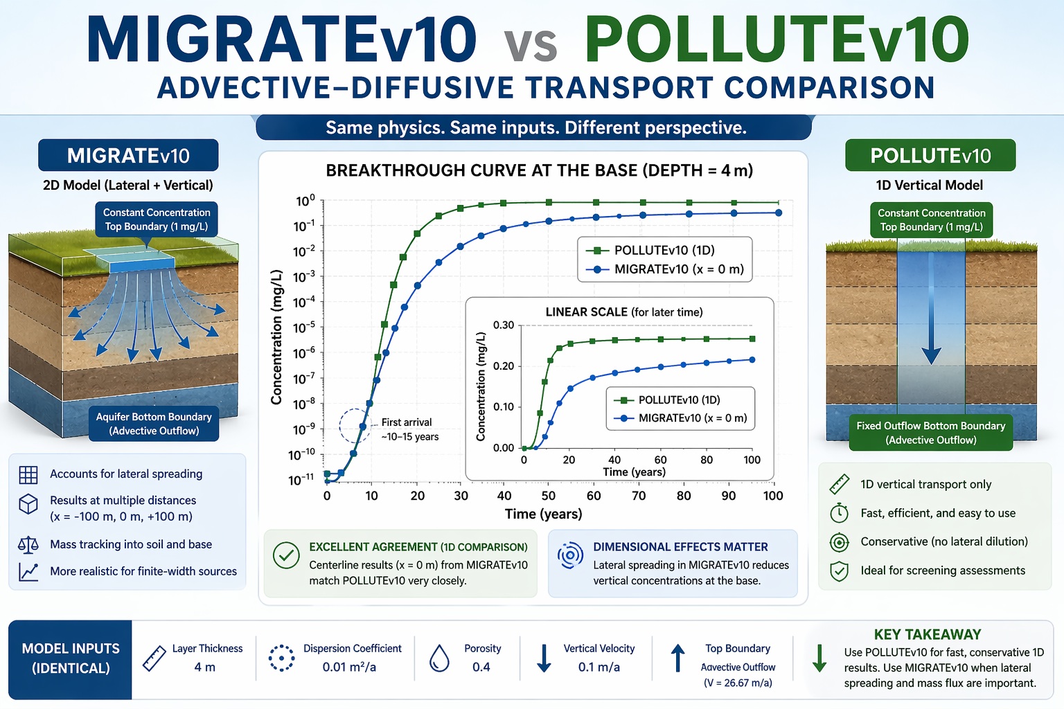
This example compares advective–diffusive transport results from MIGRATEv10 and POLLUTEv10 using identical input conditions. The goal is to evaluate consistency between the two models while highlighting key differences in how they represent contaminant transport.
Unlike pure diffusion, this case includes advection, resulting in much faster contaminant migration and earlier breakthrough at depth.
Model Setup
Both models were configured with the following parameters:
- Layer thickness: 4 m
- Diffusion/dispersion coefficient: 0.01 m²/a
- Porosity: 0.4
- Sorption: None (Kd = 0)
- Vertical velocity: 0.1 m/a
- Top boundary: constant concentration (1 mg/L)
- Bottom boundary: advective outflow (aquifer)
This represents a classic advection–dispersion problem governed by:
- Advection (bulk flow transport)
- Dispersion (spreading due to diffusion + mechanical dispersion)
Results Comparison
Concentration Profiles (Centerline Comparison)
At the centerline (x = 0 m in MIGRATEv10), results closely match POLLUTEv10.
Example: 10 Years
| Depth (m) | MIGRATEv10 (mg/L) | POLLUTEv10 (mg/L) |
|---|---|---|
| 0 | 1.001 | 1.000 |
| 1 | 1.000 | 0.9998 |
| 2 | 0.889 | 0.889 |
| 3 | 0.149 | 0.149 |
| 4 | 3.09E-05 | 2.80E-05 |
The agreement is excellent, confirming both models solve the governing equations consistently.
Key Observations
1. Rapid Downward Migration
Advection dramatically accelerates contaminant movement:
- At 5 years → plume is still developing
- At 10 years → contaminant has nearly reached the base
- At 15–20 years → most of the profile approaches source concentration
This is a major contrast to pure diffusion, where penetration is slow and gradual.
2. Breakthrough at the Base
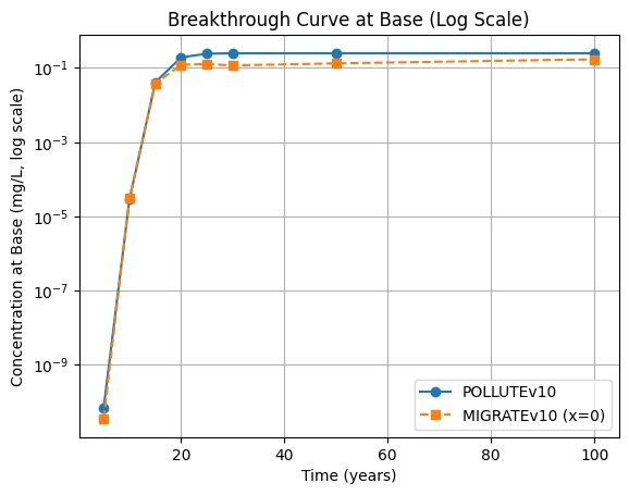
Key insights from the plot
1) Arrival time is nearly identical
- Both models show first arrival ~10–15 years
- This confirms consistent advection velocity implementation
2) POLLUTE reaches steady state faster
- Quickly approaches ~0.25 mg/L
- Represents 1D, no lateral dilution (worst-case)
3) MIGRATE predicts lower long-term concentrations
- Gradually increases to ~0.17 mg/L at 100 years
- Due to lateral spreading reducing vertical flux
4) Shape difference is important
- POLLUTE → sharp breakthrough, fast plateau
- MIGRATE → smoother rise, delayed stabilization
👉 This is a classic signature of 2D plume spreading vs 1D transport
3. Lateral Spreading (MIGRATEv10 Advantage)
MIGRATEv10 provides additional insight by modeling lateral transport.
Example: 5 Years, Depth = 1 m
| Distance | Concentration |
| x = 0 m | 0.826 mg/L |
| x = ±100 m | 0.413 mg/L |
This shows:
- Higher concentrations at the centerline
- Lower concentrations at the edges due to lateral spreading
POLLUTEv10 does not capture this effect and effectively represents the centerline (maximum concentration) case.
4. Mass Transport (MIGRATEv10 Only)
MIGRATEv10 tracks cumulative mass movement:
- At 20 years:
- Mass into soil ≈ 403
- Mass into base ≈ 85
- At 100 years:
- Mass into soil ≈ 2002
- Mass into base ≈ 1684
This demonstrates substantial contaminant flux driven by advection.
5. Boundary Condition Consistency
Although implemented differently:
- MIGRATEv10 uses an aquifer boundary with specified outflow velocity
- POLLUTEv10 uses a fixed outflow boundary
Both approaches produce equivalent results in this scenario.
Key Differences
| Feature | MIGRATEv10 | POLLUTEv10 |
| Dimensionality | 2D (lateral + vertical) | 1D (vertical only) |
| Lateral spreading | Included | Not included |
| Centerline results | Match POLLUTEv10 | Benchmark |
| Mass tracking | Yes | No |
| Use case | Finite-width sources, plume behavior | Screening-level vertical transport |
Interpretation
- POLLUTEv10 provides a conservative estimate (no lateral dilution)
- MIGRATEv10 provides a more realistic plume representation
At the centerline, both models agree. Away from the centerline, MIGRATEv10 predicts lower concentrations due to spreading.
Conclusion
This comparison shows that:
- Both models accurately simulate advective–diffusive transport
- Results are nearly identical for 1D conditions
- MIGRATEv10 extends capability to 2D systems with lateral spreading and mass tracking
For practical applications:
- Use POLLUTEv10 for fast, conservative vertical assessments
- Use MIGRATEv10 when geometry, plume shape, or mass flux are important