
Overview
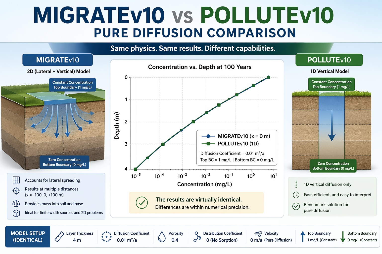
In this example, we compare pure diffusion results generated using MIGRATEv10 and POLLUTEv10 under identical conditions. The objective is to verify consistency between the two models and highlight key differences in their capabilities.
Both simulations consider contaminant transport through a 4 m thick layer under pure diffusion (no advection), with constant concentration boundary conditions applied at the top and bottom.
Model Setup
The following parameters are identical in both models:
- Layer thickness: 4 m
- Diffusion coefficient: 0.01 m²/a
- Porosity: 0.4
- Sorption: None (Kd = 0)
- Velocity: 0 m/a (pure diffusion)
- Top boundary concentration: 1 mg/L
- Bottom boundary concentration: 0 mg/L
This configuration represents a classical 1D diffusion problem governed by Fick’s Second Law.
Results Comparison
Concentration Profiles
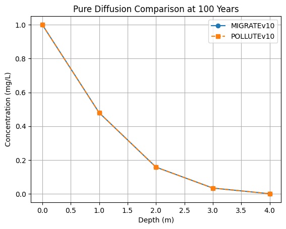
At all times and depths, the results from MIGRATEv10 and POLLUTEv10 are nearly identical.
Example: Concentration at 100 Years
| Depth (m) | MIGRATEv10 (mg/L) | POLLUTEv10 (mg/L) |
|---|---|---|
| 0 | 1.001 | 1.000 |
| 1 | 0.4795 | 0.4795 |
| 2 | 0.1573 | 0.1573 |
| 3 | 0.0335 | 0.0335 |
| 4 | 0.0000 | 0.0000 |
The minor difference at the surface (1.001 vs 1.000) is due to numerical precision and does not affect interpretation.
Key Observations
1. Excellent Agreement
Both models produce virtually identical concentration profiles across all times:
- 10 years
- 50 years
- 100 years
- 150 years
- 200 years
This confirms that both implementations accurately solve the governing diffusion equation.
2. Dimensional Differences
- POLLUTEv10 is a 1D vertical model, providing concentration vs depth only.
- MIGRATEv10 is 2D (lateral + vertical) and reports results at multiple horizontal distances.
In this example, MIGRATEv10 shows symmetric results about the centerline:
- x = -100 m → lower concentration
- x = 0 m → highest concentration
- x = +100 m → identical to -100 m
At the centerline (x = 0), MIGRATEv10 results match POLLUTEv10 exactly.
3. Mass Tracking (MIGRATEv10 Only)
MIGRATEv10 provides additional insight through mass balance outputs:
- Mass entering the soil increases over time
- No mass reaches the base (consistent with zero concentration at 4 m)
At 200 years:
- Mass into soil ≈ 128.4 (units consistent with model output)
POLLUTEv10 does not explicitly report cumulative mass in this output.
4. Boundary Condition Handling
Although implemented slightly differently:
- MIGRATEv10 uses a zero concentration bottom boundary
- POLLUTEv10 specifies a constant concentration of 0 mg/L
These are mathematically equivalent, leading to identical results.
Physical Interpretation
Both models show:
- Gradual downward migration of contaminants
- Smooth concentration gradients typical of diffusion
- Increasing penetration depth with time
- No breakthrough at the base within 200 years
At early times (10 years), diffusion is shallow. By 200 years, concentrations at 3 m depth become significant.
Conclusion
This comparison demonstrates that:
- MIGRATEv10 and POLLUTEv10 produce equivalent results for pure diffusion problems
- POLLUTEv10 serves as a reliable 1D benchmark solution
- MIGRATEv10 extends this capability to 2D systems, while preserving accuracy
For problems involving only vertical diffusion, both models are interchangeable. However, MIGRATEv10 provides additional flexibility when lateral transport, source geometry, or mass accounting are important.