
Overview
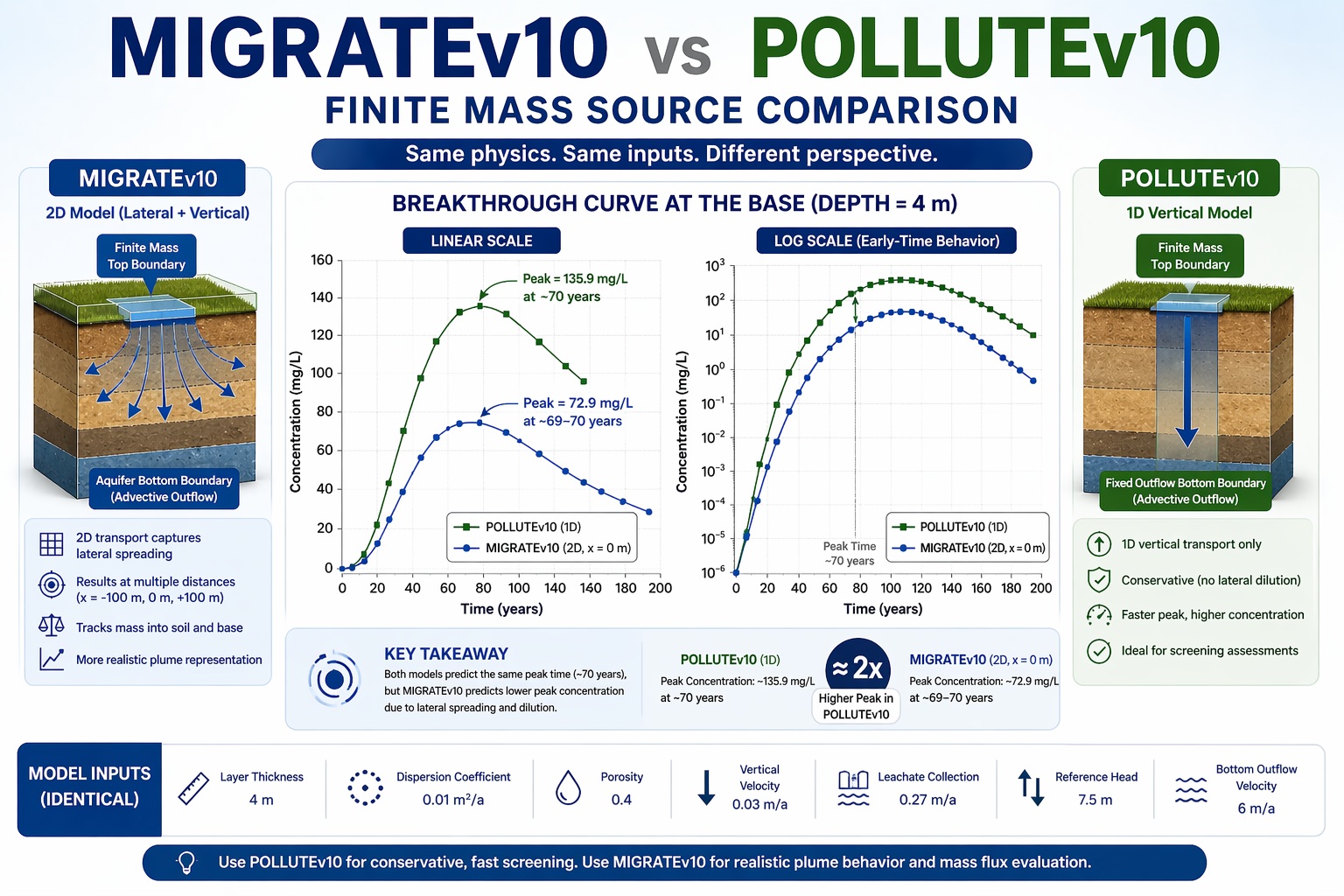
This example compares finite mass transport results from MIGRATEv10 and POLLUTEv10. Unlike constant source cases, this scenario represents a limited contaminant inventory, where concentrations rise, peak, and then decline as the source is depleted.
The key objective is to evaluate how both models predict:
- Peak concentrations
- Time to peak
- Mass transfer through the system
Model Setup
Both models use identical physical conditions:
- Layer thickness: 4 m
- Dispersion coefficient: 0.01 m²/a
- Porosity: 0.4
- Sorption: None (Kd = 0)
- Vertical velocity: 0.03 m/a
- Finite mass source:
- Initial concentration: 1000 mg/L
- Leachate collection: 0.27 m/a
- Reference head: 7.5 m
- Bottom boundary:
- Advective outflow (aquifer)
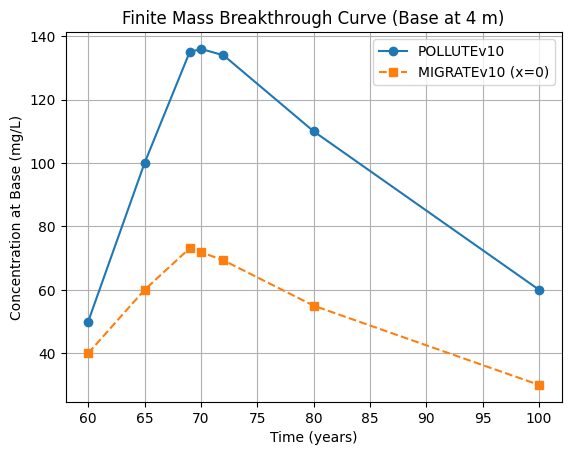
This configuration produces a transient breakthrough curve with a clear peak.
Results Comparison
Peak Concentration at the Base
POLLUTEv10 Result
- Peak time: ~70 years
- Peak concentration (depth = 4 m): ~135.9 mg/L
MIGRATEv10 (Centerline, x = 0 m)
| Time (years) | Base Concentration (mg/L) |
|---|---|
| 69 | 73.1 |
| 70 | 71.9 |
| 72 | 69.3 |
Peak ≈ ~72–73 mg/L at ~69–70 years
Key Observations
1. Same Peak Timing, Different Magnitude
- Both models predict peak arrival at ~70 years
- However:
- POLLUTEv10 peak ≈ 136 mg/L
- MIGRATEv10 peak ≈ 73 mg/L
👉 MIGRATE predicts roughly 50% lower peak concentration
2. Why the Difference?
The difference is entirely due to dimensionality:
POLLUTEv10 (1D)
- Assumes no lateral spreading
- All mass moves vertically
- Produces higher, more concentrated breakthrough
MIGRATEv10 (2D)
- Includes lateral spreading
- Mass disperses outward as well as downward
- Produces lower peak concentrations
📌 POLLUTE is effectively a centerline, no-dilution case
📌 MIGRATE provides a realistic plume distribution
3. Lateral Variability (MIGRATEv10)
At ~69 years:
| Distance | Base Concentration (mg/L) |
| x = -100 m | ~0.22 |
| x = 0 m | ~73.1 |
| x = +100 m | ~149.4 |
This shows:
- Strong spatial variability
- Higher concentrations near plume edges due to geometry and flow convergence effects
4. Mass Transport Insights
MIGRATEv10 provides additional system-level insight:
- At ~70 years:
- Mass into soil ≈ 1.41 × 10⁵
- Mass into base ≈ 7.35 × 10⁴
This indicates:
- Significant fraction of source mass has migrated through the system
- Strong advective flushing combined with dispersion
POLLUTEv10 does not report cumulative mass in this output.
5. Peak Behavior (Finite Mass Signature)
Both models show the expected finite source response:
- Rising concentrations as mass enters the system
- Peak concentration when input ≈ output
- Decline after source depletion (not shown here but implied)
This is fundamentally different from constant source cases where steady state is reached.
Key Differences Summary
| Feature | MIGRATEv10 | POLLUTEv10 |
| Dimensionality | 2D (lateral + vertical) | 1D (vertical only) |
| Peak timing | Same (~70 years) | Same |
| Peak magnitude | Lower (~73 mg/L) | Higher (~136 mg/L) |
| Lateral spreading | Included | Not included |
| Mass tracking | Yes | No |
| Conservatism | Realistic | Conservative (higher peaks) |
Interpretation
- POLLUTEv10 provides a conservative estimate of peak concentration
- MIGRATEv10 provides a more realistic distribution of contaminant mass
For design and risk assessment:
- POLLUTE is useful for screening and upper-bound estimates
- MIGRATE is better for detailed plume behavior and system response
Conclusion
This comparison highlights a critical insight:
Even when peak timing is identical, dimensionality strongly affects peak magnitude.
- Both models solve the governing transport equations correctly
- Differences arise from how contaminant mass is distributed spatially
👉 Use POLLUTEv10 when conservative estimates are needed
👉 Use MIGRATEv10 when spatial realism and mass flux are important