
Predicting the long-term environmental impact of a containment system requires more than a static model. Over decades, engineering properties change: geomembranes degrade, hydraulic heads fluctuate, and source concentrations deplete. POLLUTEv10 provides a robust “Time-Varying Properties” feature designed specifically to simulate these shifting conditions, ensuring your 1D contaminant transport models reflect real-world aging and environmental dynamics.
Why Use Time-Varying Properties?
Standard models often assume that barrier properties remain constant for the duration of the simulation. However, research shows that critical components like High-Density Polyethylene (HDPE) geomembranes undergo a multi-stage degradation process—beginning with antioxidant depletion and eventually leading to measurable changes in mechanical and hydraulic properties. By using time-varying inputs, you can accurately model:
- Geomembrane Service Life: Simulating the transition from an intact barrier to a degraded state where leakage increases significantly after a certain number of years.
- Changing Hydraulic Conditions: Adjusting hydraulic heads or velocities to account for seasonal variations or long-term climatic shifts.
- Source Concentration Decay: Reflecting how the mass of a pollutant in a landfill or pond decreases over time due to flushing or biochemical processes.
Setting Up Time-Varying Properties in POLLUTEv10
To access this features, open your model and select Time Varying Properties option on the Special Features tab. This option allows the user to vary the source concentration, reference height of leachate, volume of leachate collected, rate of concentration increase, Darcy velocity, outflow velocity, dispersivity, layer properties, and decay rate with time.
The Variable Properties option implements a “time-marching” scheme, where the program stops and restarts the solution every time parameters are changed. In the basic mode of operation the accuracy of the solution is independent of the number of sublayers. However, if the Variable Properties option is used then the accuracy of this procedure depends on the number of sublayers used in the model, and the user should experiment with the number of sublayers to ensure that the results obtained are sufficiently accurate.
Define Your Time Period
POLLUTEv10 allows you to divide your total simulation time into distinct intervals. For example, if you are modeling a landfill over 100 years, you might define:
- Years 0–15: Active operation with high hydraulic head.
- Years 15–50: Post-closure with an intact geomembrane.
- Years 50–100: Post-service life where geomembrane properties (like diffusion or permeation) are increased to simulate degradation.
When defining your time periods, consider the service lives and engineered components such as geomembranes and leachate collection systems.
Rather than a constant source, you can define a time-dependent inlet boundary condition. This is common in engineering practices where the concentration in the leachate or source pond decreases as it is depleted or diluted.
Enter the Data for each Time Period
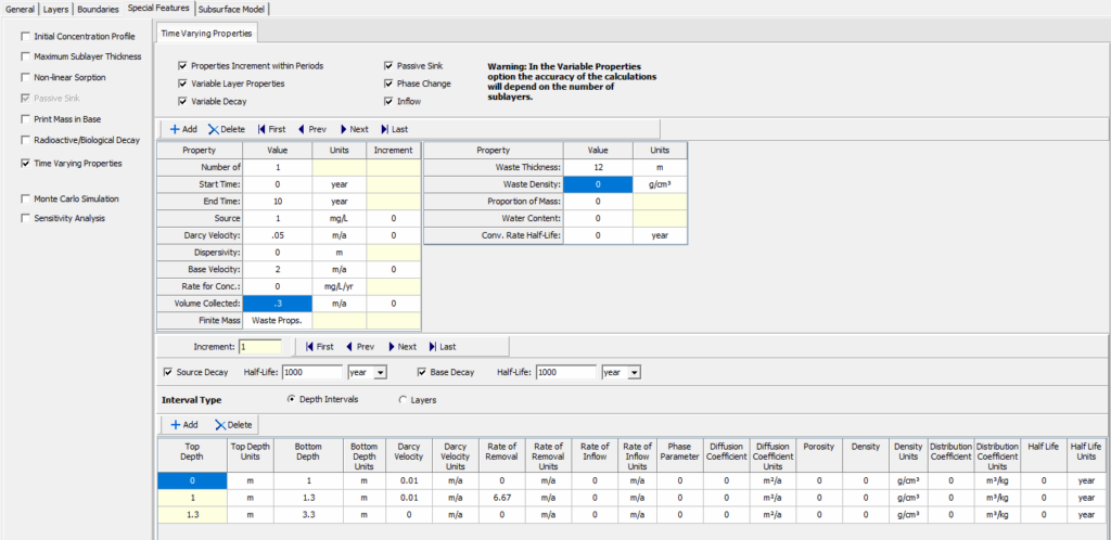
Within each time period the properties can remain constant or increment during the time period. For example, if the Darcy velocity increased linearly from .01 m/a to .11 m/a between 10 and 20 years, the user could specify 10 increments and a Darcy velocity increment of .01. If however, the properties remain constant between time periods the user need only specify the values of the properties. For example, if the Darcy velocity was .01 m/a between 0 and 10 years and then .02 m/a between 11 and 30 years, the user could specify two groups the first from 0 to 10 years with a Darcy velocity of .01 m/a and the second from 11 to 30 years with a Darcy velocity of .02 m/a.
In addition to the source varying over time, layer properties can also vary with time. Other properties that can vary with time include radioactive or biological decay, passive sinks, phase changes and inflow rates. For a detailed description of the data to be entered consult the User Guide.
Geomembrane Degradation
For geomembranes, degradation is not instantaneous. Research indicates that HDPE liners can reach their service life in as little as 8 years in some landfill operations, leading to leakage increases from 0.6 m3/d to over 27 m3/d.
When setting up your Time-Varying Properties in POLLUTEv8, selecting the right parameters for each stage of a geomembrane’s life is critical. Below is a reference table based on industry standards (such as GRI-GM13) and environmental research to help guide your inputs.
| Geomembrane Type | Stage 1 & 2: Antioxidant Depletion / Induction | Stage 3: Mechanical Failure (Cracking/Punctures) | Estimated Service Life (Years) | Typical Property Change |
|---|---|---|---|---|
| HDPE (High-Density Polyethylene) | 30 – 100+ Years | Significant increase in leakage | 100 – 400+ | |
| LLDPE (Linear Low-Density) | 20 – 60 Years | Moderate increase in diffusion | 50 – 150 | Higher initial diffusion than HDPE |
| PVC (Polyvinyl Chloride) | 10 – 30 Years | Rapid loss of plasticizer | 20 – 50 | Embrittlement leads to crack formation |
| Bituminous Geomembrane | 15 – 40 Years | Chemical oxidation | 50 – 100 | Increase in hydraulic conductivity ( |
Note: The “Service Life” varies wildly based on the exposure temperature. For example, an HDPE liner at 20 °C may last centuries, while the same liner at 60 °C (common in some industrial landfills) may reach Stage 3 in under 20 years.
Leachate Collection System Failure
A Leachate Collection and Removal System (LCRS) is the first line of defense in a modern landfill. However, as any geo-environmental engineer knows, an LCRS is not a permanent fixture. Over decades, these systems inevitably decline in efficiency due to clogging, pipe deformation, and chemical scaling.
In transport modeling, ignoring this decline leads to an underestimate of the “mounding” effect—where leachate builds up pressure (hydraulic head) against the liner, significantly increasing the risk of advective contaminant transport into the groundwater.
Why Leachate Collection Systems Fail
Even the best-engineered LCRS faces three primary “death sentences” over a 50-to-100-year period:
- Biological Clogging (Bioclogging): Microorganisms thrive in the nutrient-rich leachate, creating “slime” or biofilms that fill the void spaces in the gravel drainage layer.
- Chemical Scaling: Calcium carbonate and other minerals precipitate out of the leachate, effectively “turning the gravel to concrete.”
- Physical Silting: Fine particles from the waste mass migrate downward, even through filter layers, physically blocking the drainage paths.
The Result: The hydraulic conductivity of the drainage layer drops, the drainage pipes become less effective, and the hydraulic head acting on the underlying liner begins to rise.
Simulating LCRS Failure
To accurately model this in POLLUTEv10, you must move away from a “constant head” assumption and use the Time-Varying Properties feature.
Based on research (such as the Giroud and Houlihan equations), you can estimate how much the head will rise as the drainage layer clogs. In POLLUTEv8:
- Initial Phase (Years 0–25): LCRS is 100% functional. Set a low hydraulic head (e.g.,
).
- Transition Phase (Years 25–60): Clogging begins. Use the “Knot” feature to gradually increase the head from
to
or higher.
- Failure Phase (Years 60+): The system is effectively clogged. Model a “bathtub effect” where the head remains high or fluctuates with seasonal infiltration.
The beauty of POLLUTEv10 is the ability to synchronize failures. As the LCRS fails and the head increases, the geomembrane liner is also aging. In the Time-Varying Properties option, you can program the software so that exactly when the leachate head is at its highest, the geomembrane’s diffusion coefficient increases to reflect its “Stage 3” mechanical failure.
Summary
Using Time-Varying Properties in POLLUTEv10 transforms a simple breakthrough curve into a sophisticated lifecycle analysis. By accounting for the three stages of geomembrane degradation (antioxidant depletion, induction, and mechanical failure) and shifting hydraulic gradients, engineers can provide more accurate risk assessments for groundwater protection.
Technical Disclaimer: This guide is intended for educational purposes and provides a general overview of the capabilities of POLLUTEv10. Environmental modeling is highly sensitive to site-specific conditions and the assumptions of the user. The parameters provided in the table above are typical ranges derived from published literature and should not be used for final design or regulatory compliance without independent verification by a qualified Professional Engineer (P.Eng.) or Geoscientist. GAEA Technologies assumes no responsibility for errors, omissions, or damages resulting from the application of this information.
External Links for Further Reading
- GAEA Technologies POLLUTEv10 Documentation
- Research on HDPE Geomembrane Longevity
- Environmental Impacts of Geomembrane Aging
- Abdelaal, F.B., & Rowe, R.K. (2017). Longevity of Multi-layered Textured HDPE Geomembranes. This study provides crucial data on the antioxidant depletion stage and how solution chemistry impacts service life.
- e Silva, R.A., Abdelaal, F.B., & Rowe, R.K. (2025). A 9-year study of the degradation of a HDPE geomembrane liner. A primary source for modeling the transition between Stage I (antioxidant depletion) and Stage III (mechanical failure) over long durations.
- Rowe, R. K., et al. (1995). Diffusion of organic pollutants through HDPE geomembrane and composite liners. A foundational paper for the 1.5D advection-dispersion algorithms used in the POLLUTE software.
- Rowe, R. K. (2005). Long-term performance of contaminant barrier systems. (The 45th Rankine Lecture).
- Fleming, I. R., et al. (1999). Field observations of clogging in a landfill leachate collection system.