
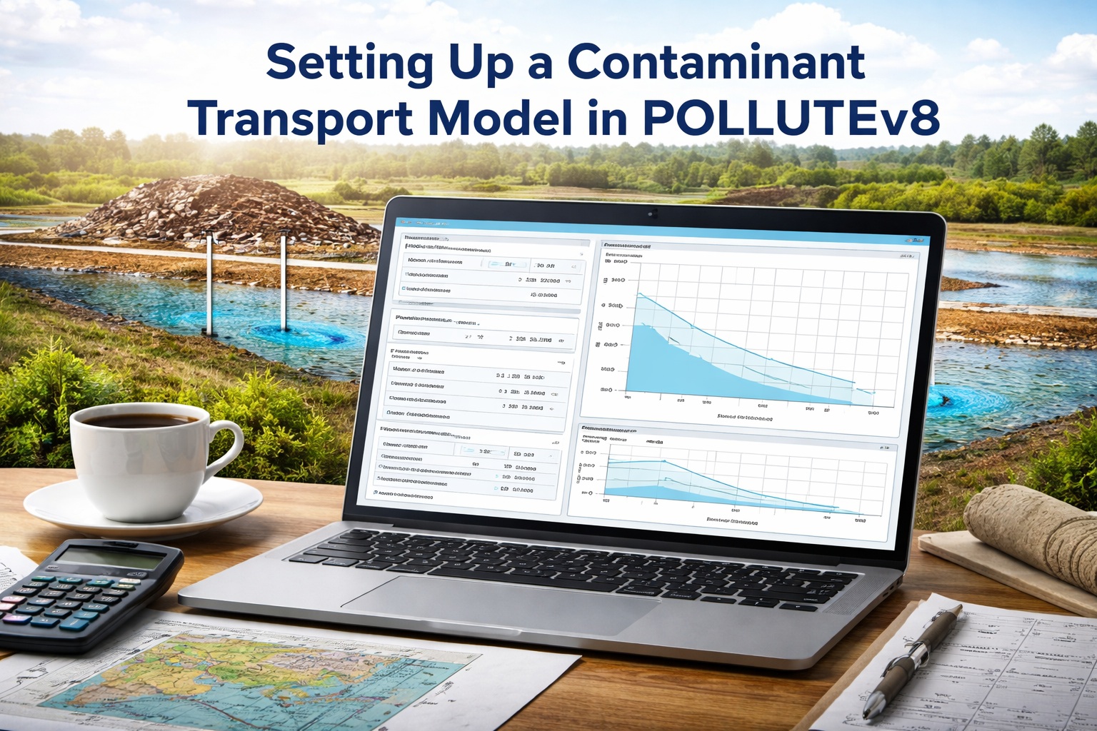
Introduction
Modeling contaminant transport in groundwater is a fundamental task in hydrogeology and environmental engineering. Whether you are assessing risks to drinking water supplies, designing remediation strategies, or evaluating plume migration, analytical tools like POLLUTEv8 provide a powerful and efficient way to simulate contaminant behavior.
POLLUTEv8 is a widely used one-dimensional analytical contaminant transport model that simulates advection, dispersion, sorption, and decay along a groundwater flow path. Its simplicity makes it ideal for screening-level assessments, regulatory support, and preliminary design studies.
This tutorial provides a complete, step-by-step guide to setting up a contaminant transport model in POLLUTEv8—from conceptualization and parameter selection to calibration and interpretation.
1. Understanding POLLUTEv8
Before building a model, it is important to understand what POLLUTEv8 does—and what it does not do.
Key Features
- One-dimensional transport along a flow path
- Analytical (not numerical) solution
- Simulates:
- Advection
- Dispersion
- Linear sorption
- First-order decay
- Supports time-varying source concentrations
When to Use POLLUTEv8
POLLUTEv8 is best suited for:
- Screening-level risk assessments
- Evaluating plume travel time
- Estimating concentrations at compliance points
- Comparing remediation scenarios
Limitations
- Assumes uniform flow conditions
- One-dimensional (no lateral spreading)
- Simplified hydrogeology
Understanding these constraints ensures appropriate use of the model.
2. Define Your Modeling Objectives
Start by clearly defining what you want the model to achieve.
Common Objectives
- Estimate contaminant concentration at a receptor well
- Determine travel time from source to compliance point
- Evaluate attenuation due to sorption and decay
- Compare remediation strategies
Example Objective
“Estimate benzene concentration 100 m downgradient over 10 years under natural attenuation conditions.”
Clear objectives guide parameter selection and model setup.
3. Develop a Conceptual Site Model (CSM)
Even for a simple analytical model, a solid conceptual understanding is essential.
Key Elements
Source Zone
- Location and extent
- Contaminant type and concentration
- Release duration
Flow Path
- Distance from source to receptor
- Groundwater velocity
- Hydraulic gradient
Aquifer Properties
- Porosity
- Dispersivity
Receptors
- Wells
- Surface water bodies
Simplification for POLLUTEv8
Because POLLUTEv8 is 1D, you must simplify the system into:
- A single flow line
- Uniform properties along that line
4. Gather Required Input Parameters
POLLUTEv8 requires a focused set of inputs. Accuracy here is critical.
Hydraulic Parameters
- Seepage velocity (v)
- Porosity (n)
Transport Parameters
- Dispersivity (α)
- Dispersion coefficient (D)
Sorption Parameters
- Distribution coefficient (Kd)
- Bulk density (ρb)
Decay Parameters
- First-order decay rate (λ)
Units must match the time scale used in the model.
Source Parameters
- Initial concentration
- Duration of release
- Time-varying input (if applicable)
5. Launch POLLUTEv8 and Understand the Interface
In POLLUTEv8 all contaminant transport models are arranged in projects. The projects can be for different landfills, contaminant sources, or areas. A new model can be assigned to an existing project or a new project.
When you open or create a model, depending on the template used for the model you will typically see input fields grouped into:
- Aquifer properties
- Transport parameters
- Source conditions
- Output controls
Take time to familiarize yourself with:
- Units used (often metric)
- Input formats
- Output options
Consistency in units is critical—double-check everything.
6. Define the Simulation Domain
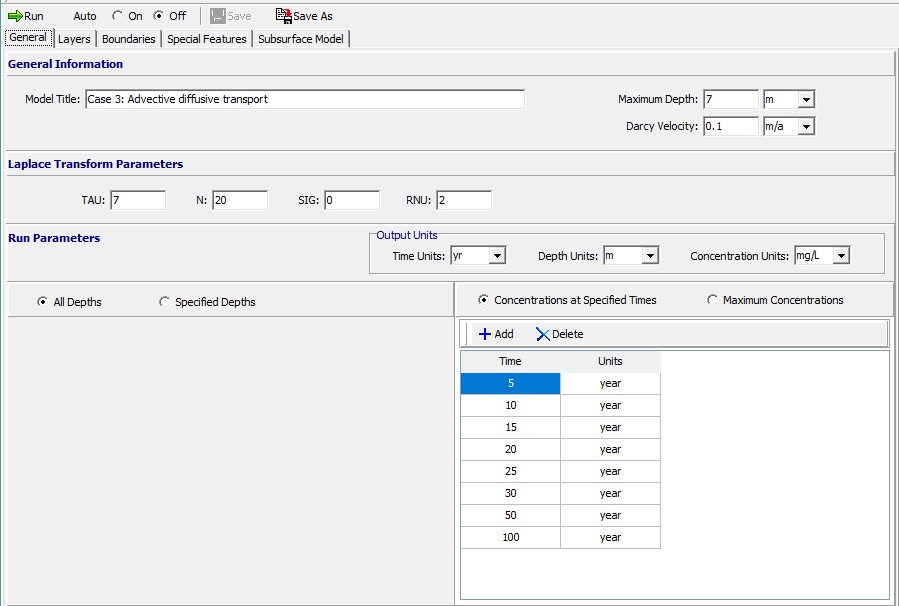
Darcy Velocity
Specify the Darcy velocity through the layers. The Darcy Velocity is defined as:
va = n*v where, n = the effective porosity, v = the seepage velocity.
If zero is entered for the Darcy velocity the transport mechanism will be purely diffusive.
Depths
The depths to calculate the concentrations can either be specified or calculated at all sublayer depths.
Times
Define the simulation times to calculate the concentrations.
Tip
If velocity is uncertain, run multiple scenarios to test sensitivity.
7. Input Layer Properties
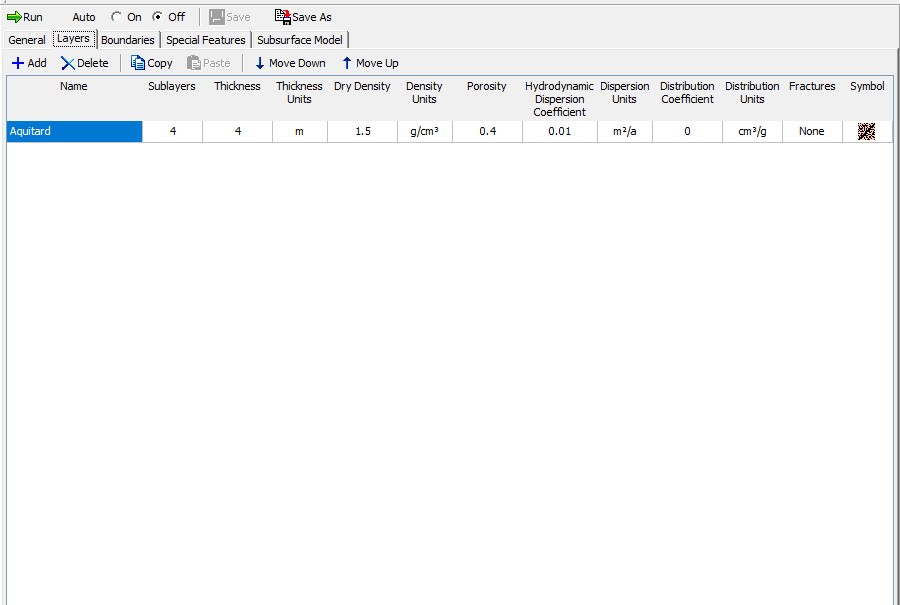
Enter the hydrogeological parameters for each layer:
- The number of sublayers in each layer is primarily used in the output of the calculated concentrations with depth; a concentration will be calculated at each sublayer interface.
- The porosity of the layer, which must be greater than 0 and less than or equal to 1. If the layer is being used to represent a geomembrane the porosity should be set to 1.
- Dry density (e.g., 1.6–2.0 g/cm³)
- The coefficient of hydrodynamic dispersion for the layer:
D = De + Dmd where, De = the diffusion coefficient for the species, Dmd = the coefficient of mechanical dispersion.
For intact clayey layers, diffusion will usually be the controlling factor and dispersion will often be negligible. In sandy layers, dispersion will tend to be the controlling factor. - The distribution coefficient for the layer. In the basic mode (ie. where Langmuir Non-linear sorption and Freundlich Non-linear sorption have not been selected) the sorption-desorption of a conservative species of contaminant is assumed to be linear such that:
S = Kd * c where, S = solute sorbed per unit weight of soil, Kd = distribution (sorption) coefficient, c = concentration of contaminant.
8. Define Boundary Conditions
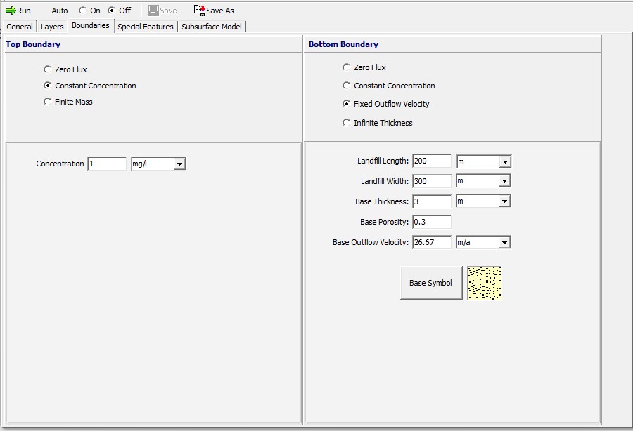
Top Boundary
- The zero flux top boundary condition represents the case where there is no transmission of contaminant across the top boundary. This option is for highly specialized applications and is rarely used.
- The constant concentration top boundary condition represents the case where the concentration of contaminant in the landfill remains constant throughout time, and is equivalent to the assumption of an infinite mass of contaminant in the landfill.
- The finite mass top boundary condition is most representative of a landfill, where the concentration of contaminant starts at an initial value, increases with time, and then declines as contaminant is transported into the subsurface and is removed by leachate collection systems.
Bottom Boundary
- The zero flux bottom boundary condition represents the case where no mass is transported into or out of the bottom of the deposit. This condition can be used to represent the case of a deposit underlain by an impermeable base stratum (e.g., intact bedrock that is impermeable relative to the overlying layer or deposit).
- The constant concentration bottom boundary condition represents the case where the concentration of contaminant remains constant in the base strata.
- The fixed outflow bottom boundary condition is most representative of the case where the model is underlain by an aquifer (permeable base strata). The concentration in the base strata (aquifer) varies with time as mass is transported into the aquifer from the deposit, and then transported away by the horizontal velocity in the base strata. The base aquifer is modelled as a boundary condition (not a separate layer) and the concentration at the bottom of the model is the concentration at the top of the base aquifer. This boundary condition assumes that there is sufficient dispersion/mixing such that the concentration is uniform across the thickness of the aquifer being considered. Thus the concentration at the bottom of the aquifer thickness modelled is the same as reported at the top of the aquifer. If the actual aquifer is very thick, normally only the upper portion (3 – 6 m depending on conditions) should be considered in modeling.
- The infinite thickness bottom boundary condition represents the case where the deposit extends infinitely in depth. This condition can be used to model lateral migration within the deposit. If the bottom boundary is specified as infinite thickness only the base symbol is required.
Real-World Consideration
If the source has stopped, simulate a finite-duration input rather than continuous loading.
9. Specify any Special Features
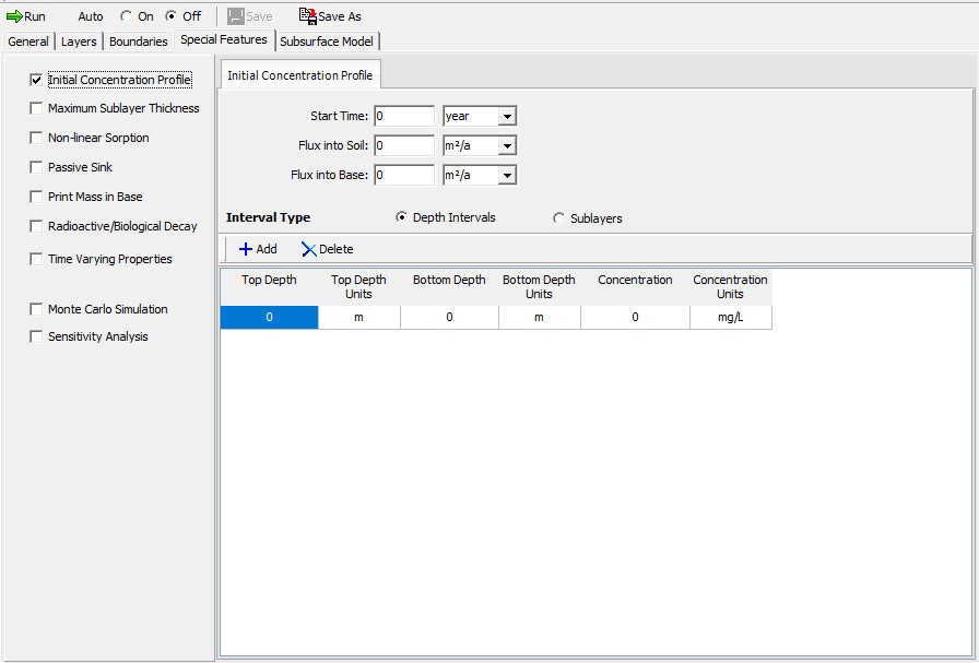
For example most models assume:
- Zero initial concentration in the aquifer
Unless historical contamination exists, this is appropriate. Otherwise, an initial concentration profile can be entered.
10. Run the Simulation
After entering all parameters:
- Review inputs carefully
- Run the model
- Check for errors or warnings
Because POLLUTEv8 uses analytical solutions, results are typically generated instantly.
11. Interpret Results
Breakthrough Curves
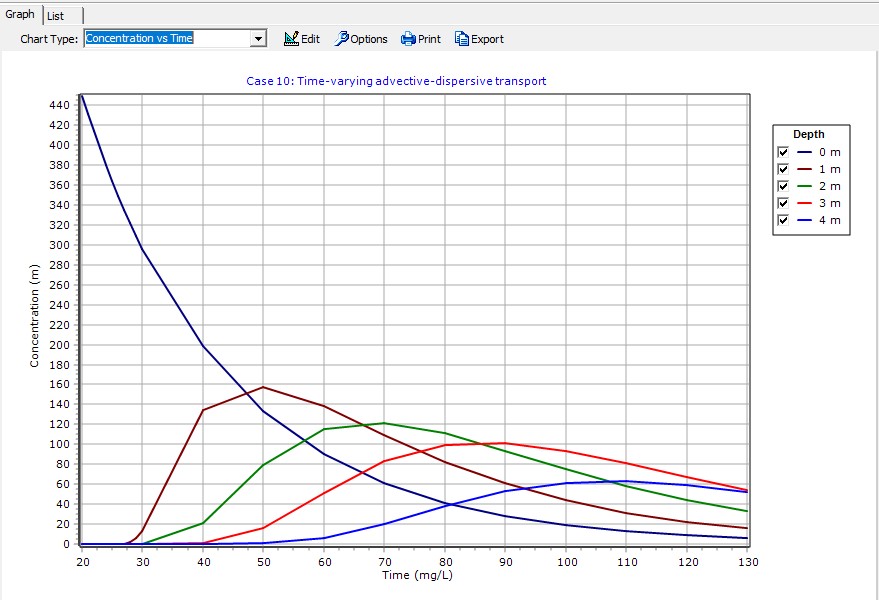
These show concentration over time at a fixed location.
Key insights:
- Arrival time
- Peak concentration
- Duration of contamination
Concentration Profiles
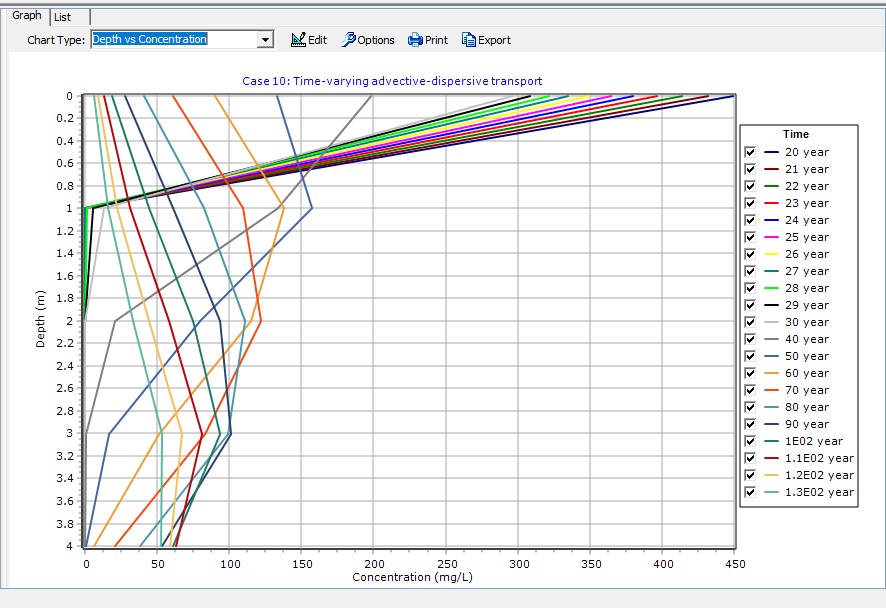
These show how the plume spreads over depth.
Look for:
- Plume length
- Attenuation trends
- Effect of dispersion
Example Interpretation
- Early arrival → high velocity
- Lower peak → strong dispersion or decay
- Delayed peak → significant retardation
12. Calibrate the Model
If field data is available, calibration improves reliability.
Compare Against:
- Monitoring well data
- Historical concentration trends
Adjust Parameters:
- Dispersivity
- Kd
- Decay rate
Important
Avoid unrealistic parameter values just to fit data—stay within reasonable ranges.
13. Perform Sensitivity Analysis
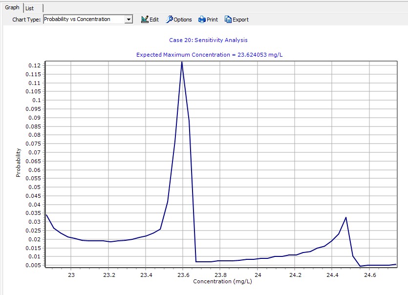
Test how sensitive results are to key parameters.
Vary:
- Velocity
- Dispersivity
- Kd
- Decay rate
Purpose
- Identify critical parameters
- Understand uncertainty
14. Run Scenario Analysis
Use the model to evaluate different conditions.
Examples
- No attenuation vs. decay
- Source removal after 1 year
- Increased groundwater velocity
Outputs
- Changes in plume length
- Reduction in concentrations
- Time to compliance
15. Common Pitfalls
Avoid these frequent mistakes:
- Incorrect units (very common)
- Unrealistic dispersivity values
- Ignoring retardation effects
- Overinterpreting a 1D model
- Using constant source when it is actually transient
16. Best Practices
- Keep the conceptual model simple and consistent
- Document all assumptions
- Use literature values as a starting point
- Validate with field data whenever possible
- Use POLLUTEv8 as a screening tool, not a final design model
Conclusion
POLLUTEv8 is a powerful yet simple tool for modeling contaminant transport in groundwater. By focusing on key processes—advection, dispersion, sorption, and decay—it allows rapid evaluation of plume behavior and risk.
By following this step-by-step workflow, you can:
- Build defensible contaminant transport models
- Estimate plume migration and concentrations
- Evaluate remediation and attenuation scenarios
- Support environmental decision-making
While POLLUTEv8 simplifies many aspects of real-world systems, its strength lies in providing fast, transparent, and interpretable results—making it an essential tool in any hydrogeologist’s toolkit.