

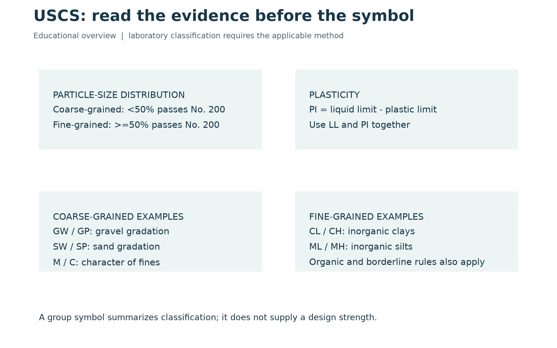
The Unified Soil Classification System, or USCS, groups soils using particle-size distribution and plasticity. Its symbols provide a compact description of classification, such as GW for well-graded gravel or CL for lean clay. The classification is useful for organizing and communicating information, but it is not a substitute for the measurements needed to design a foundation, pavement or earthwork.
A useful USCS soil classification chart should help readers follow the evidence behind a symbol. This guide explains the main branches and works through a synthetic fine-grained example. It is an educational overview rather than a reproduction of the full standard. Apply the project-specified edition of ASTM D2487 for laboratory classification and the appropriate procedure for visual-manual descriptions.
Download the reference
The geotechnical worked-examples reference (PDF) includes a simplified USCS overview, an Atterberg-limits calculation, a Proctor example and a sieve-analysis exercise. It is intended for learning and review. Borderline, organic and dual-symbol cases need the complete classification rules and supporting test information.
Begin with the fraction passing the No. 200 sieve
The main coarse-versus-fine division uses the percentage of dry mass passing the 0.075 mm, or No. 200, sieve. A soil with less than 50 percent passing is coarse-grained under this division. A soil with 50 percent or more passing is fine-grained. This is a mass-based classification decision; it should not be estimated from how much area each material occupies in a photograph.
The FHWA classification lesson illustrates this structure and the role of gradation and plasticity. An important practical consequence is that both coarse particles and fines can influence the final symbol. Calling a material sandy in a field note does not, by itself, determine its laboratory USCS classification.
Read the letters as a structured description
For coarse-grained soils, G refers to gravel and S to sand. W and P describe well-graded and poorly graded clean coarse soils. M and C describe silty and clayey fines in the relevant combinations. For fine-grained soils, common inorganic groups include ML, CL, MH and CH. L and H distinguish low and high liquid-limit groups, using the applicable boundary and chart rules.
Organic classifications require additional consideration, and highly organic material is treated separately. These distinctions are why a short symbol list cannot replace the full decision process. A chart that omits dual symbols or the borderline zone can appear simple while giving an incomplete result for a real sample. Keep the full group name, supporting measurements and classification basis together in the record.
Examine coarse-grained soils in stages
For a coarse-grained specimen, first establish whether gravel or sand predominates within the coarse fraction. Then consider the quantity and character of the fines. Clean soils require a gradation assessment; soils with more fines require information about those fines. Intermediate ranges can call for dual symbols. Use the exact thresholds and boundary conventions in the applicable standard rather than rounding a specimen into a preferred category.
Gradation is about the distribution across particle sizes. It cannot be inferred solely from the presence of both large and small particles. A grain-size curve and the necessary characteristic sizes support the evaluation. If a size needed for a calculation lies outside the measured range, do not invent it by extending the curve without a justified method. Check the laboratory procedure and whether further testing is required.
Use liquid limit and plasticity index together
For fine-grained inorganic soils, plot liquid limit on the horizontal axis and plasticity index on the vertical axis of the plasticity chart. Plasticity index is the difference between liquid limit and plastic limit. The A-line relationship commonly used in the chart is PI = 0.73(LL – 20). The liquid-limit boundary at 50 and the position relative to the A-line help distinguish the principal groups.
The chart also contains special treatment near low plasticity and for particular material types. A simple above-or-below comparison is not a complete classifier. Check whether the specimen is organic, whether the test is valid and whether it lies in a borderline region. The FHWA laboratory guide provides additional classification context; use it alongside the governing method, not as a substitute for your laboratory procedure.
Worked example: an inorganic fine-grained soil
Assume a synthetic specimen has 80 percent passing the No. 200 sieve, liquid limit 42 and plastic limit 24. Its plasticity index is 42 – 24 = 18. At LL = 42, the A-line value is 0.73 x (42 – 20) = 16.06. The point lies above that line and below a liquid limit of 50. Assuming the remaining method requirements are satisfied and the soil is inorganic, the example supports a CL group symbol.
Notice what the example does not establish. It does not supply an undrained shear strength, settlement estimate or allowable bearing pressure. Nor does it characterize every specimen from the same borehole. The calculation describes a particular hypothetical sample. When a real laboratory result is linked to a log, retain the sample identifier and interval so readers can see the scope of the evidence.
Keep field identification separate from laboratory classification
Field descriptions provide valuable observations about condition, structure and variability. They may use visual-manual identification procedures before laboratory results are available. Clearly identify that basis. A provisional field description should not become a laboratory classification merely because the same letters appear in a software selection list.
When later testing changes the classification, retain the original observation and document the revised interpretation where the project workflow requires it. Investigate major differences instead of silently replacing one label with another. Possible causes include a different sampled interval, specimen variability, an identification error or a test problem. The disagreement can reveal something useful about the data.
Avoid common chart errors
Check whether percentages refer to the whole specimen or a particular fraction. Keep units, sieve openings and preparation details visible. Do not equate clay-sized particles with clay-like plastic behaviour without considering the classification method. Avoid treating a missing plastic limit as zero or reporting a negative plasticity index as though it were an ordinary valid result.
Use consistent rounding and retain enough precision to review a boundary case. A chart should also explain its scope and source. If it is a simplified teaching diagram, label it accordingly. An attractive chart without those distinctions may encourage users to make classifications that the underlying data cannot support.
Connect the classification to a reviewable record
A complete record should identify the specimen, source location, test methods, gradation results, liquid and plastic limits, calculated index, group symbol and reviewer. That makes the classification reproducible and easier to amend if a source measurement changes. A symbol copied into a report without its supporting context is much harder to audit.
For a software walkthrough, see GAEA’s GDMS Atterberg-limits tutorial and sieve-analysis tutorial. Confirm the supported method and standard edition for your installed configuration. The most useful automation preserves the relationship between original measurements, calculations and the reviewed classification.