

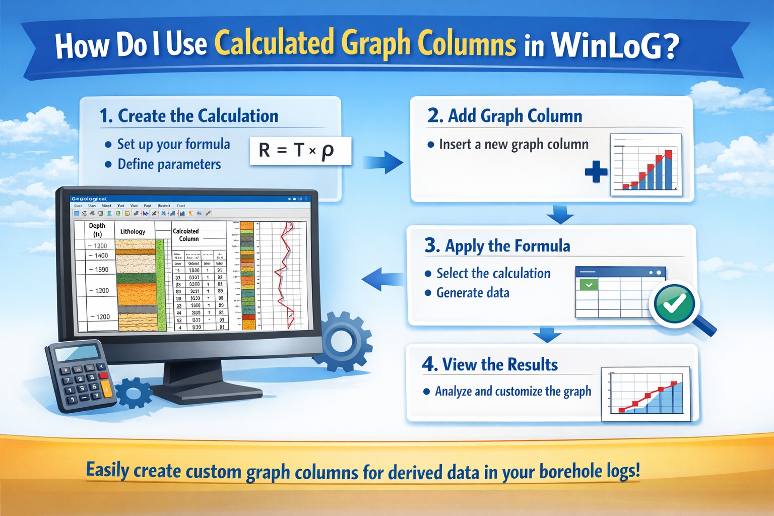
In WinLoG, calculated graph columns provide a powerful way to derive new insights from raw borehole data by applying mathematical transformations to existing datasets. These columns are particularly useful for processing geophysical logs, such as converting raw gamma readings or calculating advanced geotechnical parameters from multiple source columns.
Understanding Calculated Columns
Calculated columns function by using formulas—referred to as graph macros—to process data from one or more existing graph or geophysical datasets. For example, if a log contains two graph or geophysical datasets, A and B, a calculated column could be used to display a graph of A – 2 * B.
Creating Graph Macros
To create a calculated result, you must specify the source columns and the mathematical operation. While standard macros in other software often require complex scripting, WinLoG’ s calculated columns use a formula builder to create a graph macro.
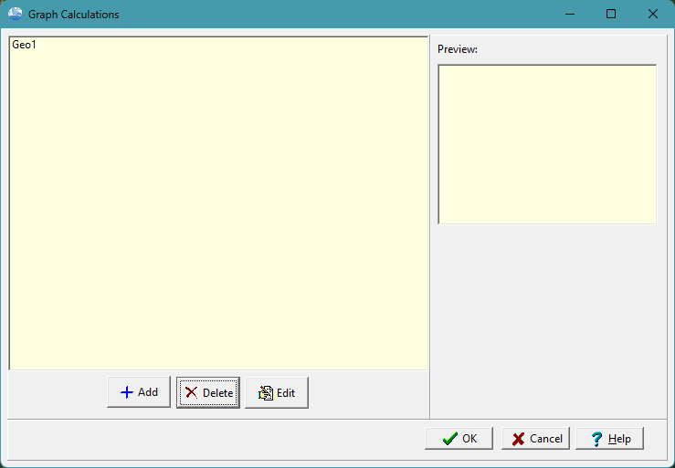
To create or edit a graph macro select Tools then Boreholes and then Graph Macros. The Graph Macro form will be displayed. On the left side of this form is a list of existing macros and on the right is the description for the selected macro. Using this form you can add a new macro or edit an existing one.
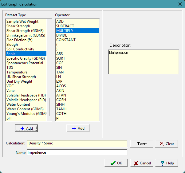
The formula for the graph macro is specified by select source columns and applying operators.
- Select Source Columns: Identify the existing graph or geophysical columns (e.g., Bulk Density and Sonic).
- Apply Operators: Use logical and mathematical operators. Common operators include:
=(Equal)< >(Not equal)+,-,*,/(Basic arithmetic)
Setting Up a Calculated Graph Column
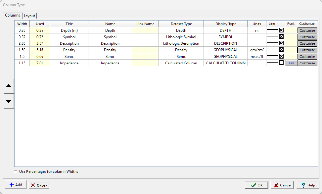
After the graph macro has been defined it can be used in a calculated graph column. To do this open the borehole template and then select Edit then Columns. Set the Dataset Type to Calculated Column and then select the Graph Macro for the Name for the column. When the template is used to create a borehole or well log, the datasets will automatically be used to calculate the column information.
Common Calculated Geophysical Curves
In geophysics, combining different data curves allows for the creation of synthetic or composite logs that provide deeper insight into subsurface properties.
The following types of geophysical curves are frequently combined:
- Sonic and Density Logs: These are commonly paired to create an Acoustic Impedance curve, which is essential for generating Synthetic Seismograms. This process helps geophysicists “tie” well log data to seismic reflection data.
- Neutron and Density Logs: This combination is standard for identifying lithology and calculating Porosity. The “crossover” between these two curves is a classic indicator of gas-bearing layers.
- Resistivity and Sonic Logs: These can be integrated to perform Source Rock Characterization. High resistivity combined with high sonic travel time often indicates the presence of organic-rich intervals.
- Gamma Ray and Resistivity/Spontaneous Potential (SP): These are often overlaid to distinguish between permeable sandstones and impermeable shales, helping to define stratigraphic boundaries and depositional environments.
- Multichannel Surface Wave (MASW) Curves: Multiple dispersion curves from different receiver spreads are combined into a mean experimental curve to increase investigation depth and improve the resolution of shear wave velocity profiles.
- Resistivity Curve “Types” (H, K, Q, A): In Vertical Electrical Sounding (VES), basic three-layer curve shapes (like H or K) are mathematically combined into complex multi-layer curves (e.g., HA, KH, or HKH) to model complex subsurface stratification.
Summary
Calculated graph columns in WinLoG streamline the transition from raw field data to finished geological reports. By leveraging macro-like formulas, users can automate the processing of geophysical logs and geotechnical test results, ensuring that derived data remains dynamic and updates automatically if the underlying source data is modified.
Related Articles
- Creating a Borehole Log from Field Data Using WinLoG and WinLoG Field Assistant
- Using Templates for Faster Borehole Logging: Standardizing Geotechnical Workflows in WinLoG
- Editing and Structuring Lithology Data: Best Practices for Accurate Borehole Logs and Geoscience Workflows
- WinLoG Advanced Features You’re Not Using (But Should)
- How Do I Create and Manage Lithologic Libraries in WinLoG?
- How Do I Create and Enter Tables in WinLoG Templates and Logs?
- How Do I Upgrade a Single User version to WinLoG Version 6?
- Moving to WinLoG v6: Seamless Data Migration for Your Borehole History
- How to use Lithology Descriptors to Standardize Logs
- How to use Sample Descriptors to Standardize Logs
- How to add Geophysical Data to a Well Log in WinLoG
- How to Quickly Enter Standardized Lithologic Layers in WinLoG
- How to Create a Well Diagram in WinLoG
- How to Import Boring and Well Data from Excel in WinLoG
- How to Import Multiple Boring and Well Locations from Excel to WinLoG
- Why is my WinLoG header data not displaying on the log?