
Landfill liner systems are designed to delay or prevent contaminant migration—but they don’t last forever. Over time, geomembranes degrade, defects grow, and hydraulic properties change. For environmental consultants, the real challenge isn’t just modeling contaminant transport—it’s accurately simulating how liner performance evolves over decades.
This is where POLLUTE stands out. Unlike many traditional models, it allows you to simulate time-varying liner failure, enabling more realistic predictions of breakthrough, long-term risk, and system performance.
In this guide, you’ll learn how to model time-dependent liner degradation step-by-step using POLLUTE.
Why Time-Varying Liner Failure Matters
Most traditional models assume liner systems are static. In reality:
- Geomembranes develop defects over time
- Hydraulic conductivity increases due to aging
- Diffusion coefficients change
- Leachate concentrations evolve
Ignoring these changes leads to:
- Underestimation of contaminant flux
- Delayed breakthrough predictions
- Inaccurate long-term risk assessments
The Key Insight
Liner performance is dynamic—not constant.
Modeling this behavior is essential for:
- Landfill design
- Regulatory submissions
- Long-term environmental impact assessment
What Is Time-Varying Liner Failure?
Time-varying liner failure refers to changes in liner properties over time, including:
- Increasing defect density
- Degradation of geomembrane integrity
- Changes in hydraulic conductivity
- Evolution of leakage rates
Instead of a single value, properties are defined as functions of time.
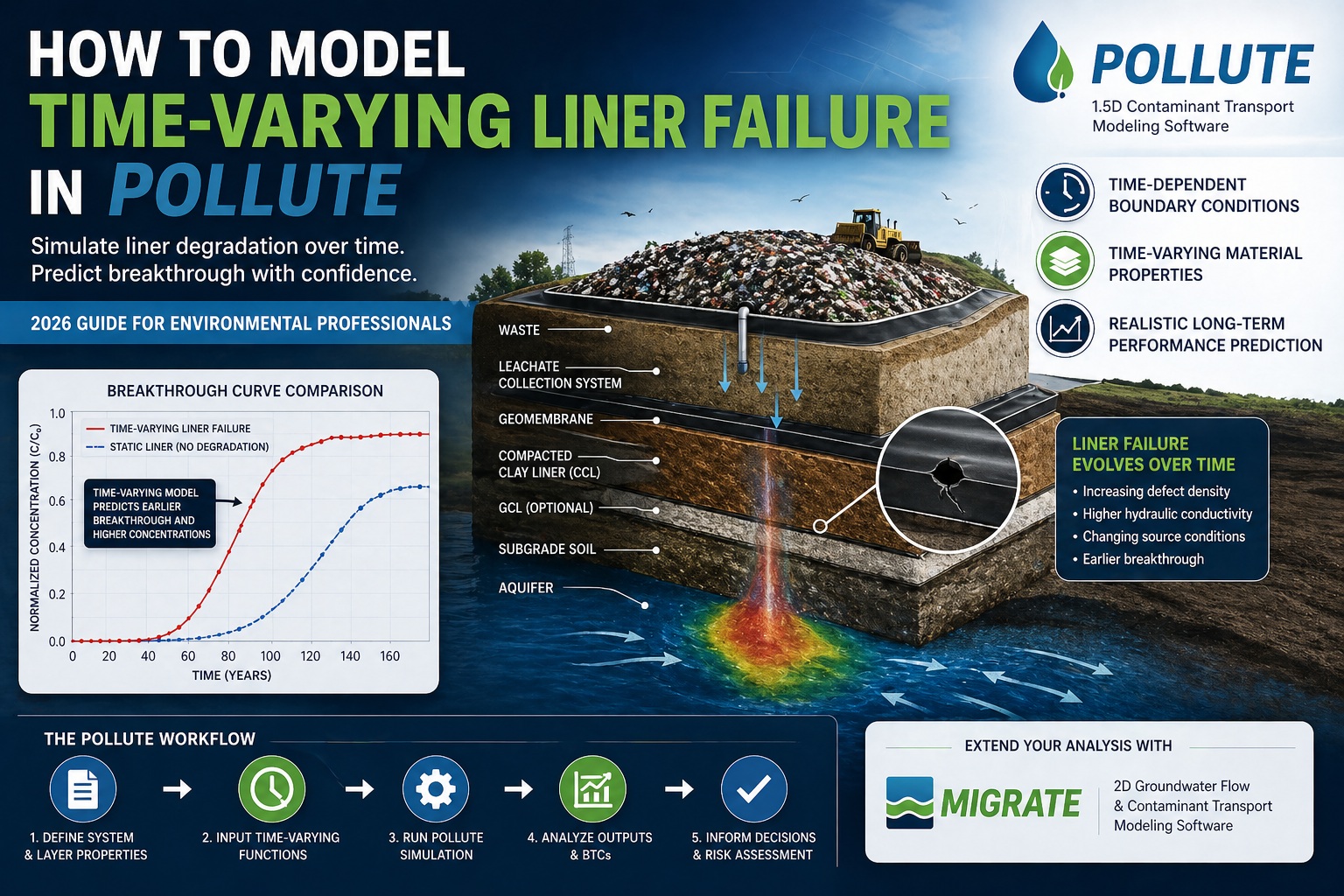
Conceptual Model of a Liner System
Before modeling, define your liner system:
Typical components include:
- Waste (source of contaminants)
- Leachate collection system (LCS)
- Geomembrane
- Compacted clay liner (CCL) or GCL
- Underlying soil/aquifer
Key Modeling Objective
Simulate how contaminants move through this system as liner performance changes over time.
Step 1: Define Initial Liner Properties
Start by entering baseline conditions into POLLUTE:
Required Inputs
- Geomembrane defect frequency
- Hydraulic conductivity of liner materials
- Thickness of each layer
- Diffusion coefficients
- Initial leachate concentration
Best Practice
Use conservative but realistic initial values based on:
- Site data
- Literature values
- Regulatory guidance
Step 2: Define Time-Varying Functions
The core of this workflow is defining how properties change over time.
Common Time-Varying Parameters
1. Defect Density
Geomembrane defects often increase due to:
- Installation damage
- Stress cracking
- Chemical degradation
Example trend:
- Year 0: 2 defects/ha
- Year 30: 50 defects/ha
- Year 100: 200 defects/ha
2. Hydraulic Conductivity
Clay liners and GCLs may degrade:
- Desiccation cracking
- Chemical interaction
- Biological activity
Result: increasing permeability over time.
3. Leachate Concentration
Source concentration is rarely constant.
It may:
- Increase during early landfill operation
- Peak during active decomposition
- Decline over time
Why POLLUTE Is Powerful Here
POLLUTE allows you to:
- Input time-dependent boundary conditions
- Define stepwise or continuous changes
- Simulate realistic degradation scenarios
Step 3: Implement Time-Varying Inputs in POLLUTE
In POLLUTE, time-varying behavior is implemented through:
1. Time-Dependent Boundary Conditions
Define how source concentration changes:
- Piecewise functions (e.g., step changes)
- Time-series input
2. Variable Material Properties
Adjust:
- Hydraulic conductivity over time
- Diffusion coefficients
- Leakage rates
3. Defect Growth Modeling
Simulate increasing leakage through geomembranes by:
- Updating defect frequency
- Adjusting equivalent leakage parameters
Step 4: Run the Simulation
Once inputs are defined:
- Run the model over the desired time frame (e.g., 100–500 years)
- Generate outputs at key depths or locations
Key Outputs
- Concentration vs. time (breakthrough curves)
- Flux through liner system
- Mass loading to aquifer
Step 5: Analyze Breakthrough Behavior
The most important result is the breakthrough curve.
C(t)
What to Look For
1. Delayed Breakthrough
Early performance may appear excellent—but degradation accelerates later.
2. Peak Shifting
Time-varying failure often shifts peak concentration forward.
3. Long-Term Tailing
Diffusion and slow release dominate after initial breakthrough.
Step 6: Compare Static vs. Time-Varying Models
To understand the impact, compare two scenarios:
Static Model
- Constant liner properties
- Predicts delayed and reduced breakthrough
Time-Varying Model (POLLUTE)
- Increasing defects and permeability
- Earlier breakthrough
- Higher peak concentrations
Key Insight
Static models often underestimate long-term risk.
Step 7: Perform Sensitivity Analysis
Time-varying models introduce uncertainty—so testing is critical.
Parameters to Vary
- Rate of defect growth
- Hydraulic conductivity increase
- Source concentration evolution
Goal
Identify which factors most influence:
- Breakthrough timing
- Peak concentration
- Long-term risk
Step 8: Model LCS Failure Scenarios
One of the most powerful applications of POLLUTE is simulating leachate collection system (LCS) failure.
Scenario Example
- Early years: efficient drainage → low head
- Later years: clogging → increased head
Impact
- Increased leakage through defects
- Accelerated contaminant transport
Result
A dramatic shift in breakthrough curve behavior.
Step 9: Integrate with Site-Wide Modeling
While POLLUTE handles vertical transport, results can be extended using:
- Site conceptual models
- 2D plume modeling tools like MIGRATE
Workflow
- Use POLLUTE to simulate liner breakthrough
- Use MIGRATE to simulate plume migration
Benefit
You capture both:
- Vertical release
- Horizontal spreading
Real-World Example
Scenario
- Composite liner system
- Time-varying leachate concentration
- Gradual geomembrane degradation
Results with POLLUTE
- Breakthrough occurs earlier than static model predicts
- Peak concentration increases over time
- Long-term tailing extends for decades
Interpretation
- Liner system delays contamination—but does not prevent it
- Long-term monitoring is essential
Common Mistakes to Avoid
1. Assuming Constant Properties
This leads to unrealistic predictions.
2. Ignoring Defect Growth
Geomembrane performance changes significantly over time.
3. Oversimplifying Source Conditions
Leachate is dynamic—model it accordingly.
4. Skipping Sensitivity Analysis
Uncertainty must be quantified.
Why POLLUTE Is Essential for This Workflow
POLLUTE is uniquely suited for modeling time-varying liner failure because it:
- Handles time-dependent boundary conditions
- Simulates multi-layer liner systems
- Supports long-term (100+ year) analysis
- Models diffusion, advection, and degradation together
Final Thoughts
Modeling time-varying liner failure is no longer optional—it’s essential for realistic environmental assessment.
The most effective approach in 2026:
- Define realistic initial liner conditions
- Model property changes over time
- Use POLLUTE to simulate breakthrough behavior
- Extend results using MIGRATE for site-wide analysis
- Validate results with field data and sensitivity testing
If you’re still relying on static assumptions, you’re likely underestimating long-term risk.
Time-varying modeling doesn’t just improve accuracy—it transforms how you understand liner performance and environmental protection over decades.