MIGRATEv10 Example 4: Finite Mass Source and Aquifer Mixing with Base Outflow

Introduction

MIGRATEv10 Example 4 builds directly on Example 3 by introducing two critical real-world complexities:

• A finite mass source (instead of constant concentration)
• An explicit aquifer boundary with flow and mixing (base outflow)

This example provides a more realistic representation of landfill behavior by simulating how a limited contaminant mass evolves over time and how it is diluted within a flowing aquifer.

⚠️ Important: This example highlights key hydrogeologic assumptions. Proper application requires expert judgment and site-specific data.

---

Conceptual Model Overview

The modeled system consists of:

• A finite mass contaminant source at the top
• A 4 m thick aquitard (low permeability layer)
• A 20 m thick aquifer (only partially modeled for mixing)

---

Key Modeling Objective

This example aims to:

• Simulate mass-limited contaminant release
• Evaluate leachate generation and migration
• Quantify dilution in the aquifer
• Demonstrate how to calculate and apply base outflow velocity (vb)

---

Source Term: Finite Mass of Waste

Unlike previous examples, the source is not infinite.

Waste Properties

Parameter	Value
Waste Thickness	6.25 m
Density	600 kg/m³
Chloride Fraction	0.2%
Peak Concentration (c₀)	1000 mg/L

• The analysis begins when peak concentration is reached
• Chloride is treated as a conservative contaminant

---

Leachate Generation

Leachate collection is defined as:

Q_c = q_o – v_a = 0.3 – 0.03 = 0.27 m/a

Where:

• ( q_o ) = infiltration through cover = 0.3 m/a
• ( v_a ) = exfiltration through base = 0.03 m/a

This represents the net leachate collected by the system.

---

Aquifer Representation

Although the aquifer is 20 m thick, only the upper 3 m is modeled.

Why?

• Full-depth mixing is unrealistic
• Mixing depends on:
  • Monitoring screen depth
  • Hydrogeologic conditions
  • Regulatory requirements

👉 Therefore:

• Modeled aquifer thickness (h) = 3 m
• Output concentration at 4 m depth represents average concentration in top 3 m

---

Flow in the Aquifer

1. Inflow to Aquifer

q{in} = v * h * L = 4 * 3 * 300 = 3600 m³/a

---

2. Flow from Landfill

q_a = v_a * L * W = 0.03 * 300 * 200 = 1800 m³/a

---

3. Total Outflow

q{out} = q{in} + q_a = 3600 + 1800 = 5400 m³/a

---

4. Base Outflow Velocity

v_b = q{out} / (W * h) = 5400 / (300 * 3) = 6 m/a

This parameter is critical because it defines how quickly contaminants are transported away in the aquifer.

---

Modeling Approach in MIGRATEv10

Step 1: Modify Example 3 Input File

• Replace constant source with finite mass source

Step 2: Define Geometry

• Aquitard thickness: 4 m
• Aquifer thickness (modeled): 3 m

Step 3: Input Source Properties

• Peak concentration: 1000 mg/L
• Define waste mass and composition

Step 4: Apply Flow Parameters

• Infiltration and exfiltration rates
• Leachate collection rate (Qc)
• Base outflow velocity (vb = 6 m/a)

Step 5: Configure Boundary Conditions

• Aquifer represented as a mixing boundary

Step 6: Run Simulation

• Track concentration over time
• Evaluate depletion of source mass
• Analyze aquifer concentrations

---

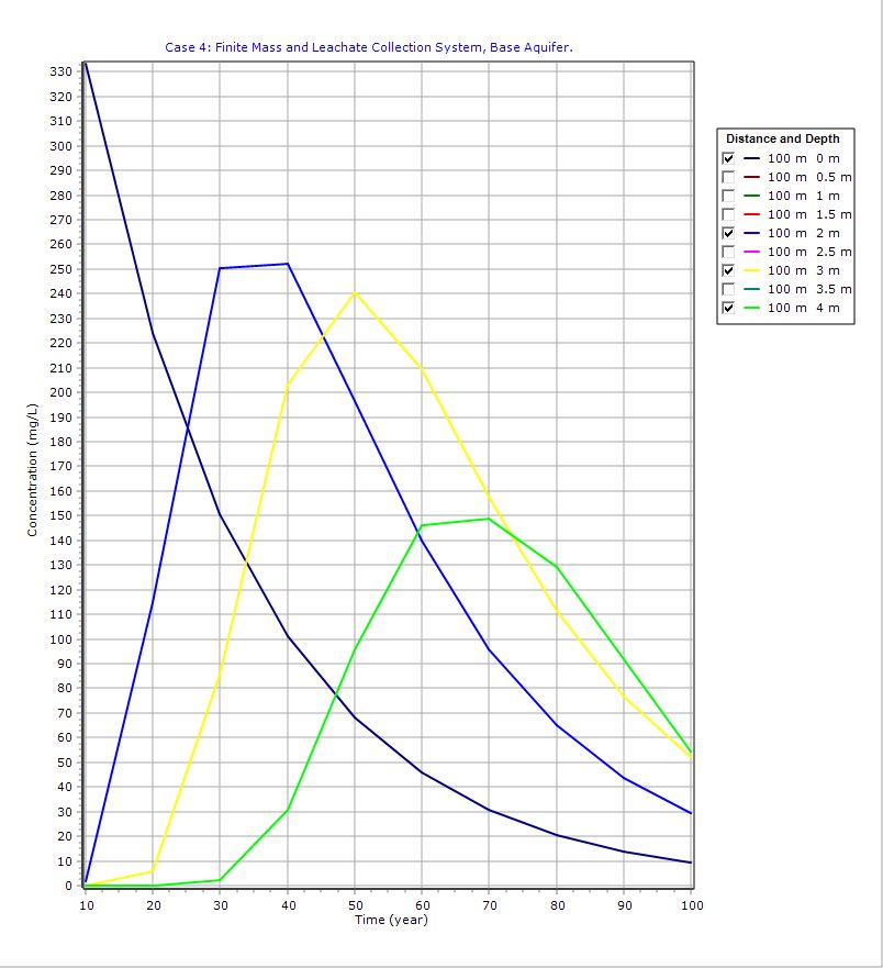
Graphical Output: Concentration vs Time

PDF Report

Interpretation of Results

1. Finite Source Behavior

• Concentrations decline over time as mass is depleted
• Unlike constant source cases, long-term impact is limited

2. Aquifer Dilution

• Concentration depends strongly on:
  • Mixing depth (h)
  • Base flow velocity (vb)

3. Sensitivity to Aquifer Thickness

• Increasing modeled thickness → lower concentrations
• Demonstrates importance of realistic assumptions

4. Role of Base Velocity

• Higher vb → faster contaminant removal
• Lower vb → greater accumulation

---

Key Takeaways

• Finite mass sources produce time-dependent contaminant release
• Aquifer mixing assumptions significantly affect results
• Base outflow velocity is a critical modeling parameter
• MIGRATEv10 allows realistic representation of mass balance and flow continuity

---

Important Warning

The calculation of base flow velocity (vb) is highly sensitive to:

• Site hydrogeology
• Landfill geometry
• Flow system changes after construction

👉 This parameter must be determined by a qualified hydrogeologist or engineer. Incorrect assumptions can lead to significant errors in predicted concentrations.

---

Final Thoughts

MIGRATEv10 Example 4 represents a major step toward realistic landfill modeling, incorporating:

• Finite contaminant mass
• Dynamic leachate generation
• Aquifer dilution and flow

This example highlights the importance of mass balance, flow continuity, and hydrogeologic context in environmental modeling.

---