
Introduction
MIGRATEv10 Example 8 introduces an important advancement in contaminant transport analysis:
👉 Evaluating concentration at multiple lateral positions
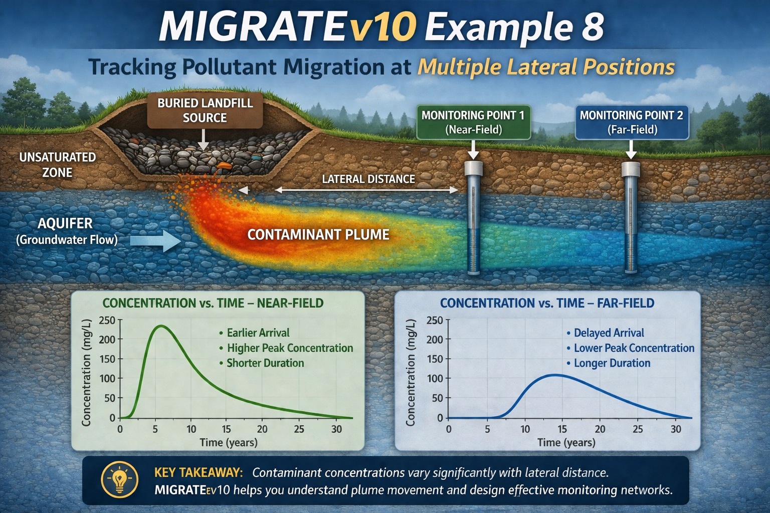
Rather than focusing on a single point, this example investigates how a pollutant migrates outward from a buried landfill and how concentrations vary at different distances from the source.
This approach provides a more realistic understanding of:
- Plume development
- Spatial variability
- Down-gradient risk
Conceptual Model Overview
The modeled system consists of:
- A buried landfill source
- Contaminant migration through subsurface materials
- An underlying aquifer system
- Multiple lateral observation points
Key Modeling Objective
The goal of this example is to:
- Calculate contaminant concentrations at two lateral positions
- Compare how plume behavior changes with distance
- Understand spatial distribution of contamination
Why Lateral Position Matters
In real-world groundwater systems:
- Contaminants do not remain directly beneath the source
- They migrate down-gradient with groundwater flow
- Concentrations vary significantly with distance and time
By analyzing multiple positions, we can:
- Track plume movement
- Identify peak concentration zones
- Evaluate compliance at monitoring locations
Modeling Approach in MIGRATEv10
Step 1: Define Source
- Buried landfill with contaminant release
Step 2: Configure Hydrogeology
- Define soil/aquifer properties
- Set groundwater flow conditions
Step 3: Select Observation Points
- Choose two lateral positions, for example:
- Near-field (close to landfill)
- Far-field (down-gradient)
Step 4: Run Simulation
- Track concentration vs time at each location
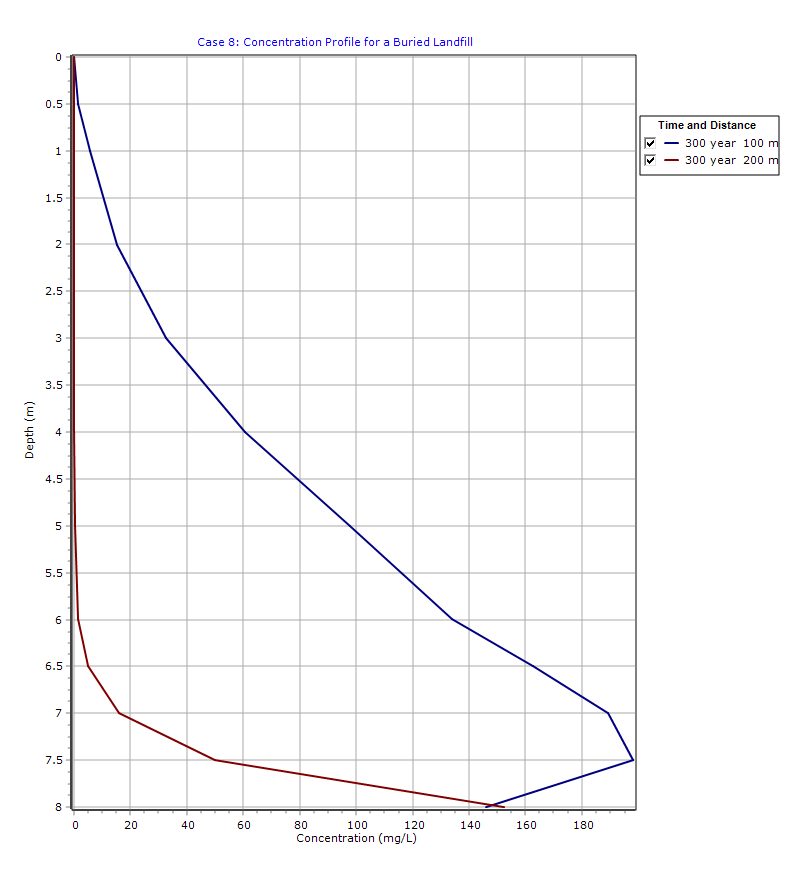
Graphical Output: Depth vs Concentration
PDF Report
 Loading…
Interpretation of Results
1. Near-Field Location
- Experiences earlier arrival of contaminants
- Higher peak concentrations
- Shorter travel time
2. Far-Field Location
- Delayed breakthrough
- Lower peak concentrations due to:
- Dispersion
- Dilution
- Broader, more spread-out plume
Typical Behavior Observed
| Characteristic | Near Source | Far from Source |
|---|---|---|
| Arrival Time | Early | Delayed |
| Peak Concentration | High | Lower |
| Plume Shape | Sharp | Broader |
| Duration | Shorter | Longer |
Key Insights
1. Plume Migration is Dynamic
The contaminant plume evolves over time and space, not just depth.
2. Distance Reduces Impact
Concentrations typically decrease with distance due to:
- Dispersion
- Mixing
- Natural attenuation (if included)
3. Monitoring Location is Critical
Results can vary significantly depending on where measurements are taken.
👉 This has direct implications for:
- Regulatory compliance
- Monitoring well placement
- Risk assessment
Practical Applications
This type of analysis is essential for:
- Designing groundwater monitoring networks
- Predicting down-gradient impacts
- Evaluating setback distances
- Supporting environmental assessments
Key Takeaways
- Contaminant concentrations vary significantly with lateral distance
- MIGRATEv10 allows evaluation of multiple observation points
- Plume behavior includes:
- Travel time
- Peak concentration
- Spatial spreading
- Understanding lateral variation is critical for real-world decision-making
Final Thoughts
MIGRATEv10 Example 8 moves beyond single-point analysis and introduces a more realistic approach to contaminant transport modeling. By evaluating multiple lateral positions, users gain a clearer picture of how pollutants migrate through groundwater systems.
This example reinforces the importance of:
- Spatial analysis
- Thoughtful monitoring design
- Interpreting results in a hydrogeologic context
Learn more about our Contaminant Transport Modeling Solutions
MIGRATE Examples
- MIGRATEv10 Example 1: Modeling a RCRA Subtitle D Landfill with a Composite Liner
- MIGRATEv10 Example 2: Composite Liner System with Primary & Secondary Leachate Collection
- MIGRATEv10 Example 3: Pure Diffusion of a Conservative Contaminant
- MIGRATEv10 Example 4: Finite Mass Source and Aquifer Mixing with Base Outflow
- MIGRATEv10 Example 5: Understanding Integration, Accuracy, and the Role of Engineering Judgment
- MIGRATEv10 Example 6: Eliminating Negative Concentrations Through Improved Integration
- MIGRATEv10 Example 7: Improving Accuracy with User-Selected Fourier Integration
- MIGRATEv10 Example 9: Comparison with the TDAST Analytical Solution
- MIGRATEv10 Example 10: Contaminant Transport in Fractured Media with Sorption
- MIGRATEv10 Example 11: Contaminant Migration from Two Adjacent Landfill Cells
- MIGRATEv10 Example 12: Modeling Time-Dependent Source Histories for Multiple Landfill Cells
- MIGRATEv10 Example 13: Termination of Primary Leachate Collection System
Comparison between POLLUTE and MIGRATE
- MIGRATEv10 vs POLLUTEv10: Pure Diffusion Comparison
- MIGRATEv10 vs POLLUTEv10: Advective–Diffusive Transport Comparison
- MIGRATEv10 vs POLLUTEv10: Finite Mass Source Comparison
- MIGRATEv10 vs POLLUTEv10: Hydraulic Trap (Finite Mass Source) Comparison
- MIGRATEv10 vs POLLUTEv10: Fractured Layer with Sorption Comparison