
Introduction
MIGRATEv10 Example 7 continues the refinement process from Examples 5 and 6 by addressing a persistent issue:
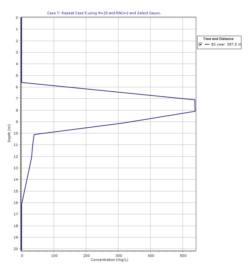
👉 Negative concentrations in the upper 5.6 m of the model domain
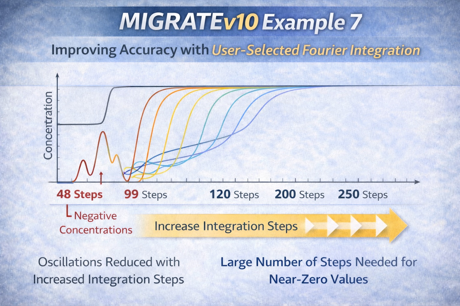
In this case, the focus shifts from Talbot integration to Fourier integration, specifically how user-selected Gauss integration parameters can significantly improve model accuracy.
This example highlights a key numerical challenge:
Accurately representing a step function using an oscillatory Fourier integral
Conceptual Overview
This example demonstrates:
- How insufficient Fourier integration leads to oscillations and negative values
- How increasing the number of integration steps improves accuracy
The Core Issue: Step Function Approximation
In this model:
- Concentrations in the upper layers behave like a step function
- MIGRATE approximates this using a Fourier integral
The Challenge
Fourier integrals are inherently:
- Oscillatory
- Prone to overshoot and undershoot (similar to Gibbs phenomenon)
👉 This can result in:
- Negative concentrations
- Poor accuracy near zero-concentration regions
Why Default Integration May Fail
Using standard settings like:
- NORMAL
- FINE
may not provide enough resolution to accurately capture the step function.
Result:
- Oscillations persist
- Negative values appear
- Concentrations near zero are poorly resolved
Solution: Increase Fourier Integration Steps
The key improvement in this example is:
👉 Using user-selected Gauss integration parameters
This allows control over:
- Number of integration steps
- Resolution of the Fourier approximation
Trial Simulations
Ten trial runs were performed using different numbers of integration steps:
| Steps | Behavior |
|---|---|
| 48 | Strong oscillations |
| 99 | Improved but still unstable |
| 120 | Reduced oscillations |
| 200+ | Significant improvement |
| 250 | Smooth and stable solution |
Graphical Output: Depth vs Concentration
PDF Report
 Loading…
Key Observation
As the number of integration steps increases:
- Oscillations decrease
- Negative concentrations disappear
- Accuracy improves—especially near zero
Important Insight
Accurate results near zero concentration require significantly more computation
This is because:
- Small values are sensitive to numerical error
- Oscillatory integrals require high resolution to stabilize
Modeling Approach in MIGRATEv10
Step 1: Identify Problem Regions
- Focus on upper 5.6 m where:
- Concentrations should be near zero
- Negative values occur
Step 2: Enable User-Defined Fourier Integration
- Switch from default settings to user-selected Gauss parameters
Step 3: Increase Integration Steps
- Test progressively higher values:
- Start ~100
- Increase to 200+ if needed
Step 4: Compare Results
- Evaluate:
- Stability
- Physical realism
- Absence of negative values
Step 5: Select Optimal Value
- Balance:
- Accuracy
- Computation time
Trade-Off: Accuracy vs Computation
| Integration Steps | Result |
| Low | Fast but inaccurate |
| Medium | Acceptable for many cases |
| High (200+) | Accurate but slower |
Key Takeaways
- Fourier integration is critical when modeling step-like concentration behavior
- Oscillations are a numerical artifact, not a physical result
- Increasing integration steps improves:
- Stability
- Accuracy
- High resolution is especially important when:
- Concentrations are near zero
- Results are sensitive
Practical Guidelines
- Use default settings for initial runs
- Increase steps when:
- Negative values appear
- Results seem unstable
- Perform a parametric study (as shown in this example)
- Don’t over-compute unless necessary
Final Thoughts
MIGRATEv10 Example 7 reinforces a critical modeling principle:
Numerical methods must be adapted to the problem being solved
When dealing with step functions and near-zero concentrations, standard settings may not be sufficient. By increasing Fourier integration steps and carefully reviewing results, users can achieve:
- Physically meaningful solutions
- Numerically stable outputs
This example is particularly important for advanced users working with:
- Sharp concentration gradients
- Boundary-driven transport
- High-precision modeling scenarios
Learn more about our Contaminant Transport Modeling Solutions
MIGRATE Examples
- MIGRATEv10 Example 1: Modeling a RCRA Subtitle D Landfill with a Composite Liner
- MIGRATEv10 Example 2: Composite Liner System with Primary & Secondary Leachate Collection
- MIGRATEv10 Example 3: Pure Diffusion of a Conservative Contaminant
- MIGRATEv10 Example 4: Finite Mass Source and Aquifer Mixing with Base Outflow
- MIGRATEv10 Example 5: Understanding Integration, Accuracy, and the Role of Engineering Judgment
- MIGRATEv10 Example 6: Eliminating Negative Concentrations Through Improved Integration
- MIGRATEv10 Example 7: Improving Accuracy with User-Selected Fourier Integration
- MIGRATEv10 Example 9: Comparison with the TDAST Analytical Solution
- MIGRATEv10 Example 10: Contaminant Transport in Fractured Media with Sorption
- MIGRATEv10 Example 11: Contaminant Migration from Two Adjacent Landfill Cells
- MIGRATEv10 Example 12: Modeling Time-Dependent Source Histories for Multiple Landfill Cells
- MIGRATEv10 Example 13: Termination of Primary Leachate Collection System
Comparison between POLLUTE and MIGRATE
- MIGRATEv10 vs POLLUTEv10: Pure Diffusion Comparison
- MIGRATEv10 vs POLLUTEv10: Advective–Diffusive Transport Comparison
- MIGRATEv10 vs POLLUTEv10: Finite Mass Source Comparison
- MIGRATEv10 vs POLLUTEv10: Hydraulic Trap (Finite Mass Source) Comparison
- MIGRATEv10 vs POLLUTEv10: Fractured Layer with Sorption Comparison