
Laboratory diffusion testing is a cornerstone of contaminant transport analysis in low-permeability soils such as compacted clays. In POLLUTEv10 Example 8, the model is applied to simulate the diffusion of potassium (K⁺) through a clay specimen under controlled laboratory conditions.
This example is based on well-established experimental work by R. Kerry Rowe and colleagues, including Michael Caers and Franco Barone, whose studies in the late 1980s helped define diffusion behavior in clay liners used in environmental containment systems.
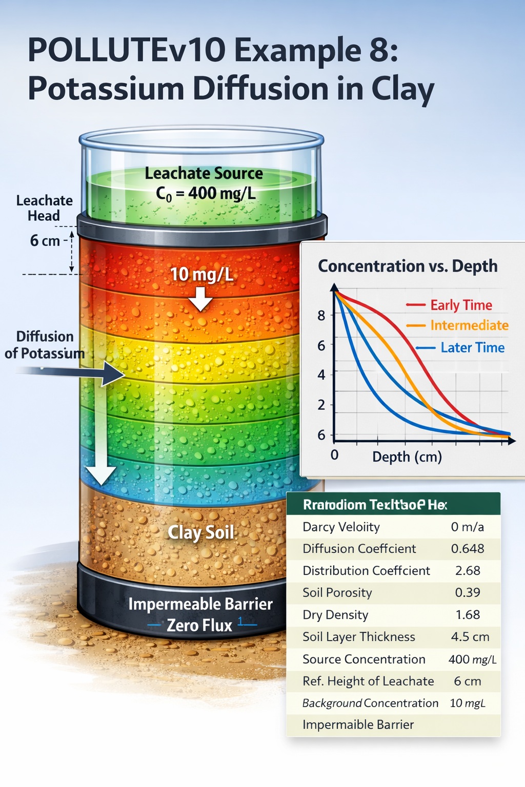
Problem Overview
The objective of this simulation is to reproduce and analyze the diffusive transport of potassium through a saturated clay layer, with the following characteristics:
- Initial background concentration in clay: 10 mg/L
- Source (leachate) concentration: 400 mg/L
- Leachate head above specimen: 6 cm
- Boundary condition at base: Impermeable (zero flux)
- Transport mechanism: Pure diffusion (no advection)
This scenario represents a closed-bottom system, commonly used in laboratory column testing to isolate diffusion processes without interference from advective flow.
Conceptual Model
The model conceptualization includes:
- A clay specimen of finite thickness
- A constant concentration source at the top boundary
- An impermeable boundary at the base (zero mass flux)
- An initial uniform background concentration throughout the clay
Since Darcy velocity is zero, transport is governed entirely by Fickian diffusion, driven by concentration gradients between the source and the clay.
Input Parameters
The following parameters are used in POLLUTEv10 for this example:
| Property | Symbol | Value | Units |
|---|---|---|---|
| Darcy Velocity | va | 0 | m/a |
| Diffusion Coefficient | D | 0.648 | cm²/d |
| Distribution Coefficient | Kd | 2.68 | cm³/g |
| Soil Porosity | nm | 0.39 | – |
| Dry Density | — | 1.68 | g/cm³ |
| Soil Layer Thickness | H | 4.5 | cm |
| Number of Sub-layers | — | 10 | – |
| Source Concentration | co | 400 | mg/L |
| Leachate Reference Height | Hr | 6 | cm |
| Background Concentration | — | 10 | mg/L |
Layer Discretization Strategy
When modeling initial concentration profiles, proper discretization is critical for numerical stability and accuracy.
In this example:
- Layer 1 (top): 0.1 cm
- Layer 2 (main body): 4.3 cm
- Layer 3 (bottom): 0.1 cm
This ensures:
- Accurate representation of boundary conditions
- Stability in modeling concentration gradients
- Proper handling of initial background concentration
The thin top and bottom layers act as buffer zones, allowing the model to better capture steep gradients near boundaries.
Key Processes Simulated
1. Diffusion
The dominant process is molecular diffusion, described by Fick’s Law. Since there is no flow:
- Transport is driven solely by concentration differences
- Movement occurs from high concentration (400 mg/L) to low concentration (10 mg/L)
2. Sorption
The distribution coefficient (Kd = 2.68 cm³/g) indicates that potassium:
- Partially sorbs onto clay particles
- Experiences retardation, slowing its migration
This reflects realistic behavior in clay liners, where cation exchange plays a significant role.
3. Boundary Conditions
- Top boundary: მუდმ constant concentration source
- Bottom boundary: Zero flux (impermeable)
This creates a one-directional diffusion system with accumulation over time.
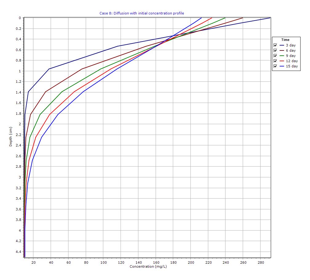
Graphical Output: Depth vs Concentration
PDF Report
 Loading…
Concentration Profiles
- Concentration decreases with depth from the source
- Over time, the diffusion front penetrates deeper into
- The bottom boundary prevents loss, causing gradual accumulation
Retardation Effects
Due to sorption:
- The effective diffusion rate is reduced
- Breakthrough at deeper layers is delayed
- Profiles show smoother gradients compared to non-reactive cases
Model Validation
This example is particularly useful for:
- Comparing POLLUTEv10 results with laboratory data
- Validating diffusion coefficients and Kd values
- Calibrating models for real-world liner systems
Practical Applications
This example has direct relevance to:
- Landfill liner design
- Contaminant migration assessments
- Environmental impact studies
- Barrier performance evaluation
Understanding diffusion in clay is essential where:
- Hydraulic conductivity is extremely low
- Long-term contaminant containment is required
Best Practices for POLLUTEv10 Users
- Always use at least three layers when defining initial concentration profiles
- Ensure thin boundary layers to improve numerical accuracy
- Verify units carefully (especially diffusion coefficients)
- Use laboratory data for calibration whenever possible
Conclusion
POLLUTEv10 Example 8 demonstrates a classic diffusion-dominated transport scenario in clay, highlighting the importance of:
- Accurate parameter selection
- Proper layer discretization
- Understanding sorption effects
By replicating laboratory conditions, this example provides a powerful tool for validating contaminant transport models and improving confidence in long-term environmental predictions.
Learn more about our Contaminant Transport Modeling Solutions
POLLUTE Examples
- POLLUTEv10 Example 1: Modeling a U.S. RCRA Subtitle D Landfill
- POLLUTEv10 Example 2: Pure Diffusion in a Soil Layer (No Sorption)
- POLLUTEv10 Example 3: Advection + Diffusion with Aquifer Mixing
- POLLUTEv10 Example 4: Finite Mass Source with Leachate Collection System
- POLLUTEv10 Example 5: Hydraulic Trap (Upward Flow into the Landfill)
- POLLUTEv10 Example 6: Fractured Layer with Sorption and Reactive Transport
- POLLUTEv10 Example 7: Lateral Migration of a Radioactive Contaminant in Fractured Rock
- POLLUTEv10 Example 9: Diffusion with Freundlich Non-Linear Sorption (Phenol in Clay)
- POLLUTEv10 Example 10: Time-Varying Advective–Dispersive Transport from a Landfill
- POLLUTEv10 Example 11: Time-Varying Source Concentration with Diffusion (Chloride in Clay)
- POLLUTEv10 Example 12: Fractured Media Transport vs Analytical Solution (Tang et al., 1981)
- POLLUTEv10 Example 13: 2D Plane Dispersion vs Analytical Solution (TDAST)
- POLLUTEv10 Example 14: Modeling a Landfill with Primary and Secondary Leachate Collection Using Passive Sink
- POLLUTEv10 Example 15: Modeling Leachate Collection System Failure Using Variable Properties and Passive Sink
- POLLUTEv10 Example 16: Monte Carlo Simulation of Leachate Collection System Failure Timing
- POLLUTEv10 Example 17: Modeling a Landfill with Composite Liners and Dual Leachate Collection Systems
- POLLUTEv10 Example 18: Modeling Phase Change in a Secondary Leachate Collection System
- POLLUTEv10 Example 19: Multiphase Diffusion of Toluene Through a Geomembrane System
- POLLUTEv10 Example 20: Sensitivity Analysis of Primary Leachate Collection System Failure