POLLUTEv10 Example 12: Fractured Media Transport vs Analytical Solution (Tang et al., 1981)

Validating Fracture Transport Modeling with Analytical Benchmarks

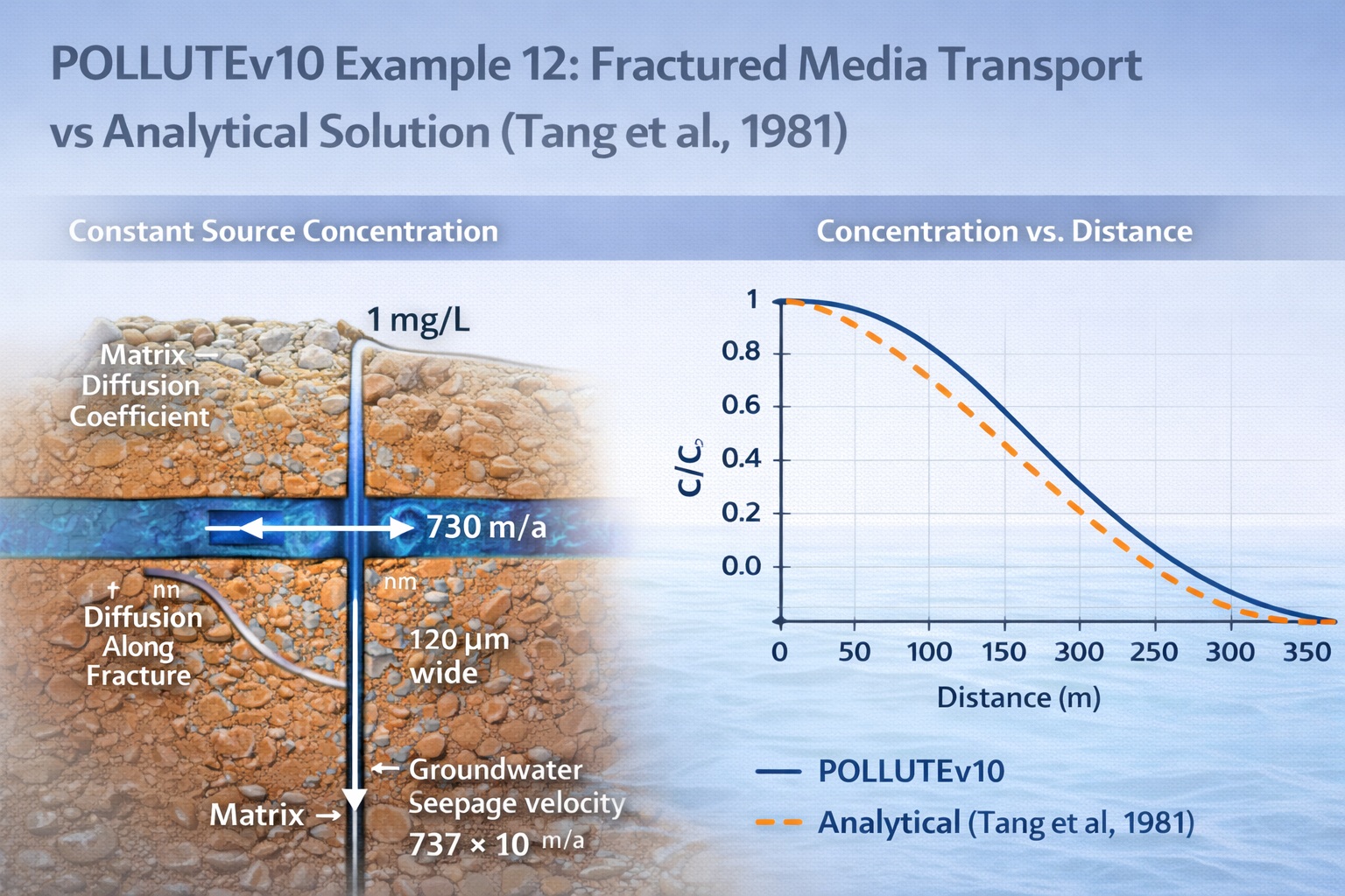
POLLUTEv10 Example 12 is a benchmark validation case that compares numerical results from POLLUTEv10 with an analytical solution developed by Tang et al..

This example focuses on transport in fractured porous media, where contaminant migration occurs rapidly along fractures and slowly into the surrounding rock matrix.

---

Problem Overview

The model simulates:

• A single fracture system
• A conservative contaminant (no sorption in fracture)
• Advection and diffusion along fractures
• Diffusion into the surrounding matrix
• A constant source concentration

Key Conditions

• Source concentration (co) = 1.0 mg/L
• Fracture spacing = 1 m
• Fracture aperture = 10 μm
• High groundwater velocity along fractures

---

Conceptual Model

The system consists of:

• Discrete fractures acting as fast-flow pathways
• A low-permeability rock matrix surrounding fractures
• Diffusion from fracture → matrix

Key Insight

Because matrix diffusion is extremely small:

There is effectively no interaction between adjacent fractures

Thus:

• Results are independent of fracture spacing over the time scale considered

---

Key Calculations

Darcy Velocity in Fractures

$$v_a = (\text{fractures per m}) \times (\text{fracture width}) \times (\text{seepage velocity})$$$$v_a = 10 \times 10^{-6} \times 1 \times 730 = 0.73 \times 10^{-2} \, \text{m/a}$$

Mix Diffusion Coefficient

$$D_m = D_f \times \text{tortuosity}$$$$D_m = 0.077 \times 0.0000983 = 7.57 \times 10^{-6} \, \text{m}^2/\text{a}$$

---

Input Parameters

Property	Value	Units
Darcy Velocity (va)	0.73E-2	m/a
Soil Thickness (H)	400.0	m
Sub-layers	4	–
Fracture Spacing	1.0	m
Fracture Opening	10E-6	m
Fracture Diffusion Coefficient	0.077	m²/a
Fracture Distribution Coef.	0.0	cm³/g
Matrix Diffusion Coefficient	7.57E-6	m²/a
Matrix Distribution Coef.	1.0	cm³/g
Matrix Porosity (nm)	0.05	–
Dry Density (Matrix)	0.0	g/cm³
Source Concentration	1.0	mg/L

---

Transport Mechanisms

1. Advection in Fractures

• Rapid contaminant movement
• Dominant transport pathway

2. Diffusion Along Fractures

• Spreads contaminant longitudinally
• Controlled by Df = 0.077 m²/a

3. Matrix Diffusion

• Very slow transfer into surrounding rock
• Controlled by low tortuosity

4. No Dispersion

• Dispersivity = 0
• Simplifies comparison with analytical solution

---

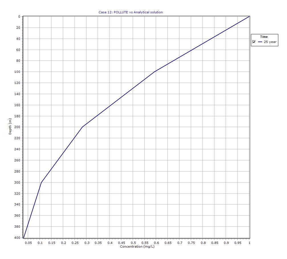
Graphical Output: Depth vs Concentration

---

PDF Report

Key Insights

• Fractures dominate contaminant transport in rock
• Matrix diffusion can be negligible depending on tortuosity
• Analytical solutions are valuable for model validation
• POLLUTEv10 accurately simulates dual-porosity systems

---

Importance of Model Setup

Even though only 4 sub-layers are used:

• Large domain (400 m) simplifies gradients
• Low matrix interaction reduces complexity

However:

More layers may be required for higher precision or stronger matrix interaction

---

Practical Applications

This example is critical for:

• Fractured rock aquifer analysis
• Nuclear waste repository studies
• Contaminant transport in bedrock
• Model verification and calibration

---

Conclusion

POLLUTEv10 Example 12 demonstrates the model’s ability to accurately simulate fracture–matrix transport systems and match established analytical solutions.

Key takeaways:

• Fracture flow controls transport speed
• Matrix diffusion may be minimal in some systems
• Analytical comparisons are essential for validation

This example builds confidence in using POLLUTEv10 for complex fractured media problems.

---