POLLUTEv10 Example 3: Advection + Diffusion with Aquifer Mixing

Share the knowledge

This example builds directly on Example 2 by introducing advective transport and a permeable aquifer boundary. This scenario is much closer to real-world landfill hydrogeology, where both diffusion and groundwater flow control contaminant migration.

Overview of the Scenario

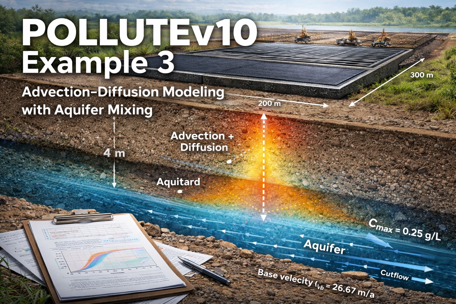
In this example, the system consists of:

A 4 m thick aquitard (low permeability layer)
A constant contaminant source at the top (landfill)
A 3 m thick active aquifer zone (upper portion of a 20 m aquifer)
Downward flow (advection) through the aquitard
Mixing in the aquifer controlled by flow continuity

Key Enhancements from Example 2:

✅ Advection included (va ≠ 0)
✅ Aquifer explicitly represented as a boundary
✅ Flow continuity used to calculate dilution
❌ Still no sorption (Kd = 0)

Conceptual Model

The transport system includes:

Downward advection + diffusion through aquitard
Mass transfer into aquifer at 4 m depth
Dilution in flowing groundwater system

The aquifer is treated as a well-mixed receptor zone, not a full 3D domain.

Input Parameters

Property	Symbol	Value	Units
Darcy Velocity	va	0.1	m/a
Diffusion Coefficient	D	0.01	m²/a
Distribution Coefficient	Kd	0	cm³/g
Soil Porosity	n	0.4	–
Dry Density	ρd	1.5	g/cm³
Aquitard Thickness	H	4	m
Sub-layers	–	4	–
Source Concentration	c₀	1	g/L
Landfill Length	L	200	m
Landfill Width	W	300	m
Aquifer Thickness	h	3	m
Aquifer Porosity	nb	0.3	–
Base Outflow Velocity	vb	26.67	m/a

Governing Transport Equation

With both advection and diffusion:

$\frac{\partial C}{\partial t} + v_a \frac{\partial C}{\partial x} = D \frac{\partial^2 C}{\partial x^2}$ ∂t∂C+va∂x∂C=D∂x2∂2C

This equation shows:

Advection term (va ∂C/∂x) → dominates transport
Diffusion term (D ∂²C/∂x²) → smooths gradients

Flow Continuity Calculations

A key part of this example is determining the aquifer dilution using flow balance.

1. Inflow to Aquifer (Upgradient)

$q_{in} = v_{in} \cdot h \cdot W = 20 \cdot 3 \cdot 300 = 18000 \, m^3/a$

2. Flow from Landfill (Recharge)

$q_a = v_a \cdot L \cdot W = 0.1 \cdot 200 \cdot 300 = 6000 \, m^3/a$

3. Total Outflow

$q_{out} = q_{in} + q_a = 18000 + 6000 = 24000 \, m^3/a$

4. Base Outflow Velocity

$v_b = \frac{q_{out}}{W \cdot h} = \frac{24000}{300 \cdot 3} = 26.67 \, m/a$

Peak Concentration (Hand Calculation)

Because advection dominates, the peak aquifer concentration can be estimated:

$c_{max} = \frac{q_a \cdot c_0}{q_{out}}$

$c_{max} = \frac{6000 \cdot 1}{24000} = 0.25 \, g/L$

✔ Key Insight:

The aquifer concentration is controlled by dilution, not diffusion
This provides a quick validation check against model results

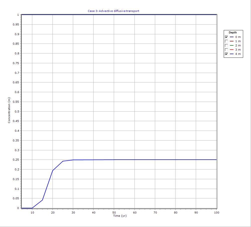
Graphical Output: Concentration vs Time

PDF Report

Loading…

Taking too long?

Reload document

Open in new tab

Key Results

Peak aquifer concentration: 0.25 g/L
Transport dominated by advection
Dilution governed by flow continuity

Conclusions

Advection significantly increases contaminant migration rate
Aquifer dilution is critical in determining impact
Simple hand calculations can approximate peak concentrations
Model highlights importance of accurate hydrogeologic characterization

Engineering Warning

The parameter vb (base outflow velocity) must be carefully evaluated:

Depends on:
- Aquifer transmissivity
- Hydraulic gradients
- Landfill recharge
In complex systems:
- Numerical groundwater models may be required
- Simple continuity assumptions may not be sufficient

Key Engineering Insights

This example bridges the gap between:
- Pure diffusion (Example 2)
- Real-world transport systems
Demonstrates:
- Importance of flow systems
- Sensitivity to Darcy velocity
- Role of aquifer thickness in dilution