Phenol Diffusion with Freundlich Sorption Explained

Share the knowledge

In POLLUTEv10 Example 9, the model advances beyond linear sorption by incorporating Freundlich non-linear sorption to simulate the diffusion of phenol through a clay specimen. This example reflects more realistic contaminant behavior, particularly for organic compounds that do not follow simple linear partitioning.

Problem Overview

This example simulates a laboratory diffusion test with the following conditions:

Contaminant: Phenol
Soil: Clay (7 cm thick)
Transport mechanism: Diffusion only (no advection)
Sorption model: Freundlich non-linear isotherm
Bottom boundary: Impermeable (zero flux)
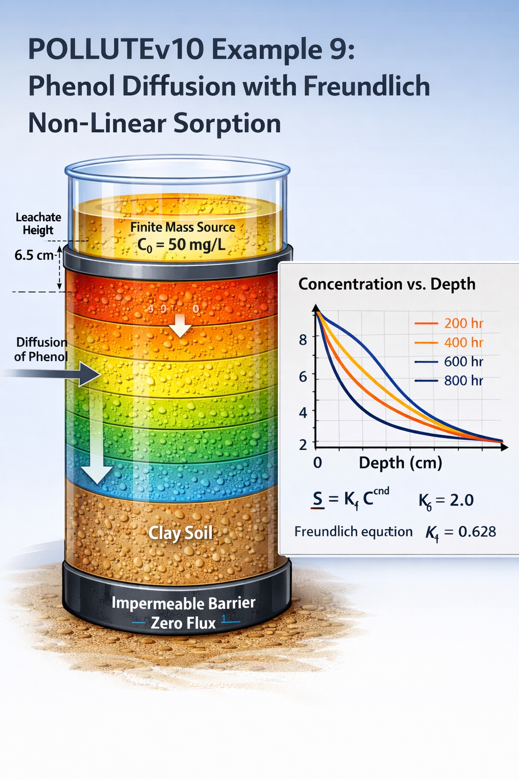
Source type: Finite mass

Source Conditions

Initial concentration (co): 50 mg/L
Leachate head (Hr): 6.5 cm

Times of Interest

200 hr
400 hr
600 hr
800 hr

Conceptual Model

The system consists of:

A finite mass source of phenol at the top
A clay layer where diffusion and sorption occur
An impermeable base preventing downward flux

Unlike constant concentration sources, the finite source means:

Concentration at the top decreases over time
Transport is influenced by both diffusion and depletion

Input Parameters

Property	Symbol	Value	Units
Darcy Velocity	va	0.0	cm/hr
Diffusion Coefficient	D	0.019	cm²/hr
Freundlich Coefficient	Kf	2.0	cm³/g
Sorption Exponent	—	0.628	–
Soil Porosity	n	0.46	–
Dry Density	—	1.47	g/cm³
Soil Layer Thickness	H	7.0	cm
Number of Sub-layers	—	14	–
Source Concentration	co	50.0	mg/L
Leachate Height	Hr	6.5	cm

Understanding Freundlich Non-Linear Sorption

The Freundlich isotherm describes sorption as:

$S = K_f \, C^n$

Where:

S = sorbed concentration
C = լուծ dissolved concentration
K_f= sorption capacity
n = non-linearity exponent

Key Implications

Sorption is not constant (unlike linear Kd models)
Retardation varies with concentration
Transport becomes concentration-dependent

With n = 0.628 (< 1):

Sorption is stronger at lower concentrations
This causes tailing effects in concentration profiles

Key Processes Simulated

1. Diffusion

Governed by concentration gradients
Slower compared to Example 8 due to lower diffusion coefficient

2. Non-Linear Sorption

Phenol interacts with clay via Freundlich behavior
Retardation is dynamic, not constant

3. Finite Mass Source

Source concentration decreases over time
Results in attenuated diffusion fronts

4. Boundary Condition

Zero flux at base → contaminant accumulates within the domain

Importance of Layer Discretization

This example highlights a critical modeling requirement:

Accuracy depends strongly on the number of sub-layers when using non-linear sorption.

Why?

Non-linear equations require finer resolution
Concentration-dependent retardation must be captured precisely
Coarse discretization can lead to numerical errors

Best Practice

Use ≥ 14 sub-layers (as in this example)
Increase layers further for higher accuracy or steeper gradients

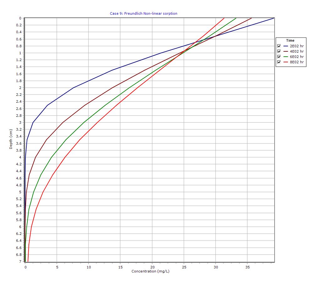
Graphical Output: Depth vs Concentration

PDF Report

Loading…

Taking too long?

Reload document

Open in new tab

Concentration Profiles

Profiles evolve over time (200 → 800 hr)
Slower migration compared to conservative solutes
Gradual flattening due to source depletion

Non-Linear Effects

Stronger sorption at low concentrations causes extended tails
Profiles are non-symmetric and more complex

Finite Source Behavior

Peak concentrations decrease over time
Diffusion front weakens as source mass is exhausted

Practical Applications

This example is especially relevant for:

Organic contaminant transport (e.g., phenol, hydrocarbons)
Landfill leachate assessments
Clay liner performance evaluation
Risk assessment modeling

It is particularly important when:

Contaminants exhibit non-linear adsorption
Long-term predictions are required
Laboratory calibration data is available

Best Practices for POLLUTEv10 Users

Always verify Freundlich parameters (Kf and n) from lab data
Use fine discretization for non-linear problems
Compare results at multiple time steps
Be cautious when interpreting retardation (not constant!)

Conclusion

POLLUTEv10 Example 9 demonstrates how incorporating Freundlich non-linear sorption significantly enhances the realism of contaminant transport modeling.

Key takeaways:

Non-linear sorption leads to concentration-dependent transport
Finite sources introduce time-varying boundary conditions
Numerical accuracy depends heavily on layer discretization

This example is essential for modeling organic contaminants in clay systems, where linear assumptions are often insufficient.

Learn more about our Contaminant Transport Modeling Solutions

POLLUTE and MIGRATE Contaminant Modeling and Landfill Design

POLLUTEv10 Example 9: Diffusion with Freundlich Non-Linear Sorption (Phenol in Clay)

Knowledge Center