POLLUTEv10 Example 4: Finite Mass Source with Leachate Collection System

Introduction

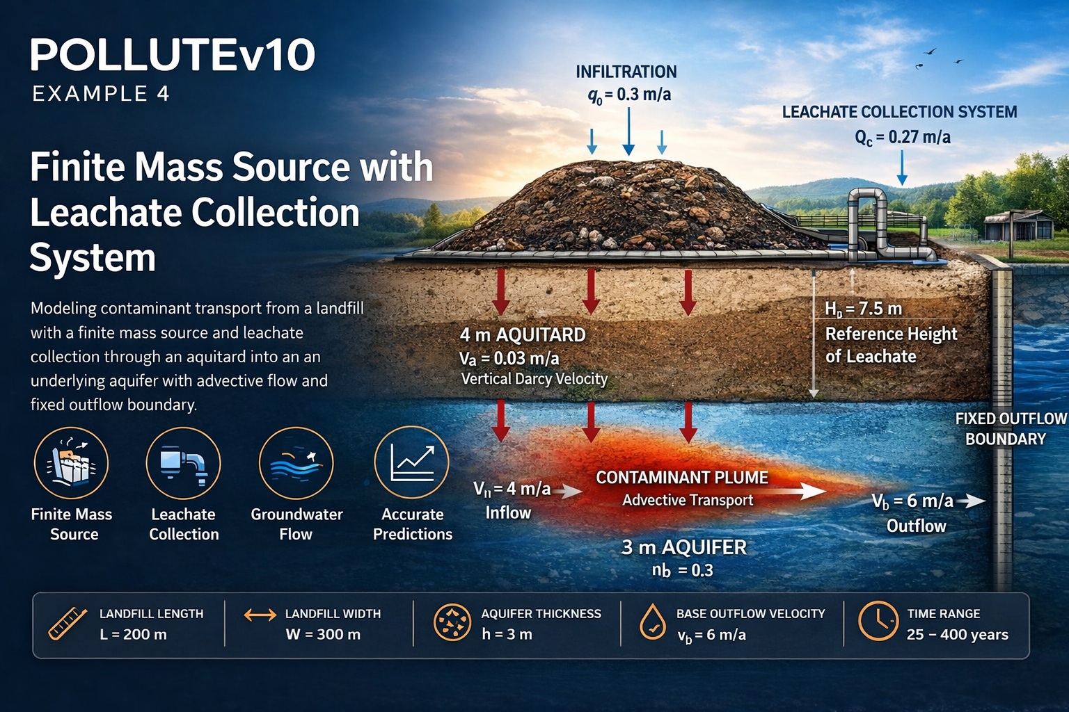
This example builds directly on the conceptual and numerical framework established in Case 3, introducing a more realistic landfill condition: a finite mass contaminant source combined with an active leachate collection system. This scenario better reflects modern engineered landfills, where contaminant release is limited by waste mass and partially controlled through collection infrastructure.

The model simulates contaminant migration from a landfill through a low-permeability layer into an underlying aquifer, while accounting for declining source mass and reduced leachate flux due to collection.

---

Conceptual Model Overview

The hydrogeological system remains consistent with Case 3, with the following structure:

• A 4 m thick upper soil layer (aquitard)
• A finite mass contaminant source at the surface (landfill)
• A 3 m thick aquifer beneath
• A fixed outflow boundary at the downgradient edge

Key Enhancements in Example 4:

• Finite contaminant mass instead of constant concentration
• Inclusion of a leachate collection system
• Adjusted groundwater velocities
• Time-dependent source behavior (though constant in this case due to assumptions)

---

Landfill Geometry and Hydrogeology

Parameter	Symbol	Value	Units
Landfill Length	L	200	m
Landfill Width	W	300	m
Aquifer Thickness	h	3	m
Aquifer Porosity	nb	0.3	–
Base Outflow Velocity	vb	6	m/a
Time Range	t	25–400	years

Important Note:
The landfill width (W) is perpendicular to groundwater flow and does not influence results in this 2D model.

---

Finite Mass Source Calculation

Unlike previous examples, the contaminant source is defined by a finite mass of chloride within the waste.

Step 1: Total Chloride Mass per Unit Area

$m_{tc} = 0.002 \times 600 \times 6.25$

Where:

• Chloride fraction = 0.2% (0.002)
• Waste density = 600 kg/m³
• Waste thickness = 6.25 m

Result:

• $m_{tc} = 7.5 \, \text{kg/m}^2$

---

Step 2: Reference Height of Leachate (Hr)

$H_r = \frac{m_{tc}}{c_0}$

Where:

• $c_0 = 1000 \, \text{mg/L} = 1 \, \text{kg/m}^3$

Result:

• $H_r = 7.5 \, \text{m}$

---

Step 3: Rate of Increase in Concentration (Cr)

Because peak concentration is reached early:

• Cr = 0 mg/L/a

This simplifies the model by eliminating time-dependent concentration buildup.

---

Leachate Collection System

A key addition in this example is the leachate collection system, which reduces contaminant loading to the subsurface.

Leachate Collection Rate

$Q_c = q_o – v_a$

Where:

• $q_o = 0.3 \, \text{m/a}$ (infiltration through cover)
• $v_a = 0.03 \, \text{m/a}$ (vertical Darcy velocity)

Result:

• $Q_c = 0.27 \, \text{m/a}$

This indicates that most infiltrating water is captured, significantly reducing contaminant migration.

---

Groundwater Flow Conditions

Upgradient Inflow Velocity:

• $v_{in} = 4 \, \text{m/a}$

Downgradient Outflow Velocity:

$v_b = v_{in} + \frac{v_a L}{h}$

Substituting values:

• $v_b = 4 + \frac{0.03 \times 200}{3} = 6 \, \text{m/a}$

This ensures mass balance across the system.

---

Transport Parameters

Property	Symbol	Value	Units
Vertical Darcy Velocity	va	0.03	m/a
Diffusion Coefficient	D	0.01	m²/a
Distribution Coefficient	Kd	0	cm³/g
Soil Porosity	n	0.4	–
Dry Density	ρd	1.5	g/cm³
Soil Thickness	H	4	m
Sub-layers	–	4	–
Source Concentration	co	1000	mg/L
Rate of Increase	cr	0	mg/L/a
Ref. Height	Hr	7.5	m
Leachate Collected	Qc	0.27	m/a

---

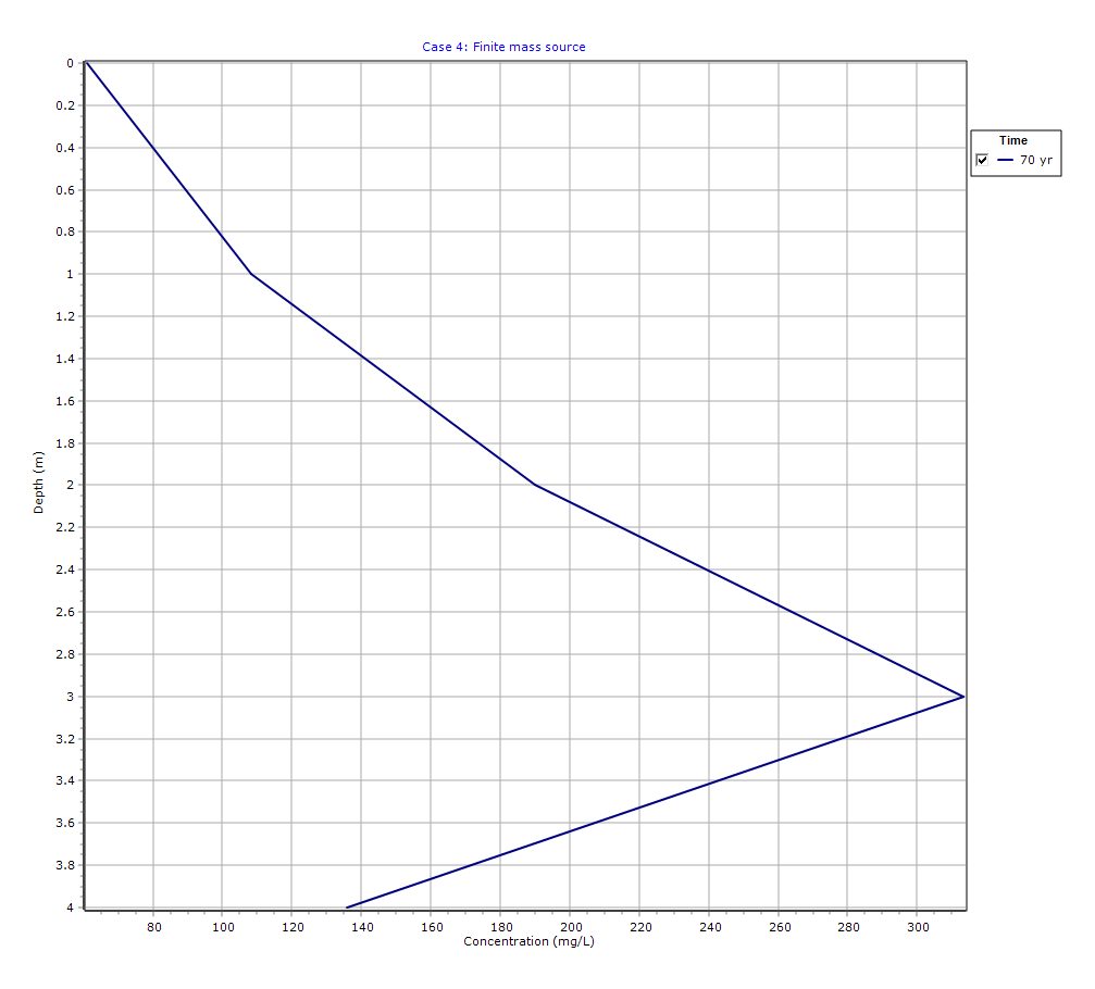
Graphical Output: Depth vs Concentration

PDF Report

Interpretation of Results

This example highlights several important hydrogeological and modeling insights:

1. Finite Source Behavior

Unlike constant concentration models, the finite mass source:

• Limits total contaminant release
• Results in eventual depletion of the source
• Produces more realistic long-term predictions

2. Impact of Leachate Collection

The collection system:

• Reduces downward contaminant flux
• Decreases plume concentration and extent
• Represents modern landfill engineering controls

3. Advective Transport Dominance

With:

• Horizontal velocity = 4 m/a
• Vertical velocity = 0.03 m/a

Transport is strongly horizontal in the aquifer, leading to plume elongation downgradient.

---

Practical Applications

This modeling scenario is particularly relevant for:

• Landfill design and risk assessment
• Regulatory compliance modeling
• Evaluation of leachate collection efficiency
• Long-term contaminant fate predictions
• Phase II Environmental Site Assessments (ESA)

---

Key Takeaways

• Finite mass sources provide realistic contaminant release behavior
• Leachate collection significantly reduces environmental impact
• Proper velocity balancing ensures accurate groundwater modeling
• POLLUTEv10 can simulate complex engineered landfill systems

---