
Introduction
MIGRATEv10 Example 5 is less about a specific landfill configuration and more about how to use the model intelligently. It emphasizes two critical aspects of contaminant transport modeling:
- The importance of engineering judgment and preliminary estimates
- The role of numerical integration accuracy in obtaining reliable results
This example highlights that modeling is not just about running software—it’s about understanding when results can be trusted and when additional effort is required.
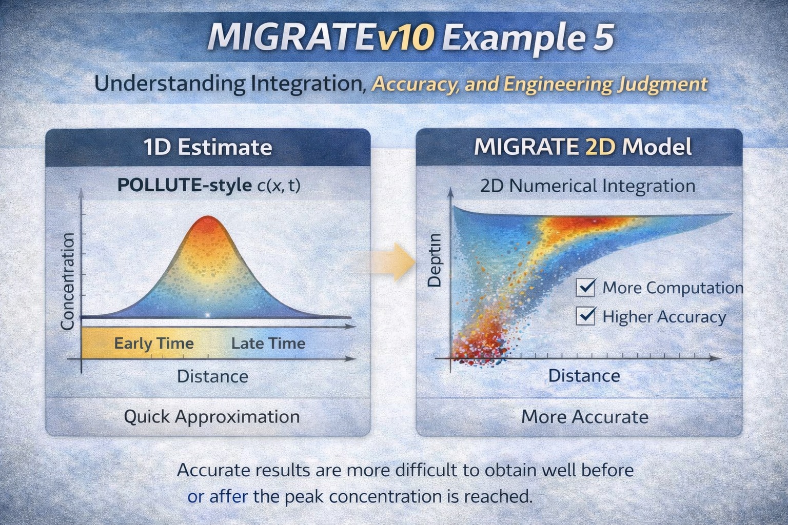
Conceptual Overview
This example compares:
- 1-D analytical-style estimates (quick, approximate)
- 2-D numerical modeling (MIGRATEv10) (more accurate, more computational effort)
Key Modeling Insight #1: Start with a 1-D Estimate
Before running a full MIGRATE simulation, users should:
- Estimate the travel time of the contaminant front
- Or estimate the position of the front at a given time
Why This Matters
A quick 1-D approximation (e.g., using tools like POLLUTE-style solutions) helps:
- Verify that model results are reasonable
- Provide a baseline expectation
- Identify potential setup errors early
👉 MIGRATE (2-D) should be used to refine, not replace, this initial understanding.
Key Modeling Insight #2: 2-D Models Require More Computation
MIGRATEv10 uses numerical integration techniques, including:
- Fourier integration
- Talbot integration
Because MIGRATE solves 2-D transport, it involves:
- Double integration
- Increased computational complexity
- Longer run times
When More Integration Is Needed
Default integration settings are often sufficient—but not always.
Increase Integration Parameters When:
- Concentrations are very small
- (e.g., long before or after peak arrival)
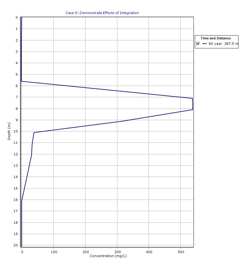
- Negative concentrations appear
- Negative flux values are calculated
👉 These are clear indicators of numerical instability or insufficient integration resolution
Recognizing Inaccurate Results
One of the key takeaways from this example:
Incorrect results are usually obviously incorrect
Warning Signs in Output
- Negative concentration values
- Oscillating or unrealistic trends
- Non-physical flux behavior
When these occur:
- Increase Fourier or Talbot terms
- Re-run the simulation
- Compare results
Peak Concentration Behavior
Accurate results are easiest to obtain:
- Near the peak concentration
More difficult to compute:
- Long before the peak arrives
- Long after the peak has passed
Why?
Because:
- Concentration gradients are small
- Numerical precision becomes critical
- Integration must resolve very small values
Practical Modeling Workflow
Step 1: Perform a 1-D Estimate
- Approximate travel time or plume location
- Use analytical or simplified tools
Step 2: Run MIGRATEv10 (2-D Model)
- Use default integration parameters initially
Step 3: Review Results Critically
- Check for:
- Negative values
- Unrealistic trends
Step 4: Refine Integration
- Increase:
- Fourier terms
- Talbot parameters
Step 5: Perform a Parametric Check
- Run multiple simulations with higher settings
- Confirm results are stable
Graphical Output: Depth vs Concentration
PDF Report
 Loading…
Why This Example Is Important
This example reinforces that:
- Models are tools—not answers
- Numerical methods require careful validation
- Computational efficiency must be balanced with accuracy
It also highlights a key principle:
Good modeling starts with understanding the physics, not just running software
Key Takeaways
- Always start with a simple 1-D estimate
- MIGRATE’s 2-D solution provides greater accuracy but requires more computation
- Integration parameters control numerical precision
- Negative values are a clear sign of model issues
- Additional computation is often required for:
- Early-time predictions
- Late-time predictions
Final Thoughts
MIGRATEv10 Example 5 is a reminder that modeling is as much an art as it is a science. While the software provides powerful tools for simulating contaminant transport, the responsibility lies with the user to:
- Validate assumptions
- Check results critically
- Adjust parameters when needed
By combining engineering judgment, simple analytical estimates, and advanced numerical modeling, users can produce results that are both accurate and defensible.
Learn more about our Contaminant Transport Modeling Solutions
MIGRATE Examples
- MIGRATEv10 Example 1: Modeling a RCRA Subtitle D Landfill with a Composite Liner
- MIGRATEv10 Example 2: Composite Liner System with Primary & Secondary Leachate Collection
- MIGRATEv10 Example 3: Pure Diffusion of a Conservative Contaminant
- MIGRATEv10 Example 4: Finite Mass Source and Aquifer Mixing with Base Outflow
- MIGRATEv10 Example 6: Eliminating Negative Concentrations Through Improved Integration
- MIGRATEv10 Example 7: Improving Accuracy with User-Selected Fourier Integration
- MIGRATEv10 Example 8: Evaluating Contaminant Migration at Multiple Lateral Positions
- MIGRATEv10 Example 9: Comparison with the TDAST Analytical Solution
- MIGRATEv10 Example 10: Contaminant Transport in Fractured Media with Sorption
- MIGRATEv10 Example 11: Contaminant Migration from Two Adjacent Landfill Cells
- MIGRATEv10 Example 12: Modeling Time-Dependent Source Histories for Multiple Landfill Cells
- MIGRATEv10 Example 13: Termination of Primary Leachate Collection System
Comparison between POLLUTE and MIGRATE
- MIGRATEv10 vs POLLUTEv10: Pure Diffusion Comparison
- MIGRATEv10 vs POLLUTEv10: Advective–Diffusive Transport Comparison
- MIGRATEv10 vs POLLUTEv10: Finite Mass Source Comparison
- MIGRATEv10 vs POLLUTEv10: Hydraulic Trap (Finite Mass Source) Comparison
- MIGRATEv10 vs POLLUTEv10: Fractured Layer with Sorption Comparison