
Introduction
MIGRATEv10 Example 3 presents a simplified but highly instructive case of pure diffusion of a conservative contaminant through a porous medium. Unlike previous examples, this scenario excludes:
- Advection (no groundwater flow in the modeled layer)
- Sorption (no retardation effects)
This makes it an ideal example for understanding the fundamental physics of diffusion-controlled transport in subsurface environments.
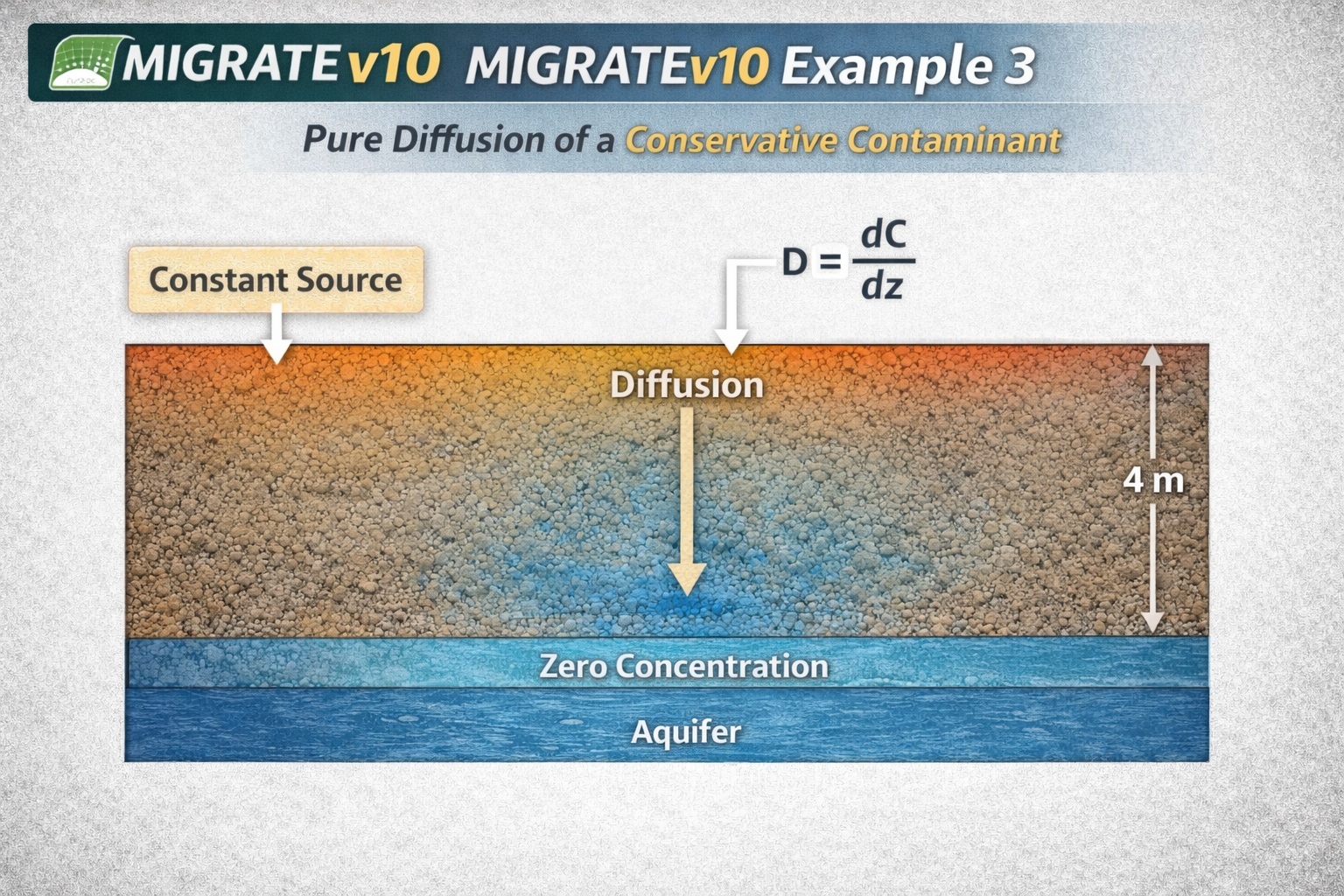
Conceptual Model Overview
The modeled system consists of:
- A 4 m thick homogeneous layer
- A constant concentration source at the top boundary
- An underlying aquifer acting as a zero-concentration boundary
Key Simplification
The aquifer is not explicitly modeled because:
- It has a high flushing velocity
- Any contaminant reaching it is immediately removed
- Therefore, concentration at the base is assumed to be zero
Key Modeling Objective
The purpose of this example is to:
- Demonstrate diffusion-driven transport
- Understand concentration gradients over time
- Provide a baseline case for comparison with more complex models
Hydrogeologic Concept
Boundary Conditions
| Boundary | Condition |
|---|---|
| Top of Layer | Constant concentration |
| Bottom of Layer | Zero concentration |
This creates a concentration gradient, which drives diffusion downward.
Governing Process: Diffusion
Transport is governed entirely by Fick’s Law of Diffusion, where contaminant flux is proportional to the concentration gradient.
- Movement occurs from high concentration → low concentration
- No influence from flow or chemical interactions
Key Assumptions
- Conservative contaminant (no decay, no sorption)
- Homogeneous porous medium
- One-dimensional vertical transport
- Steady boundary conditions
- Instantaneous removal at aquifer boundary
These assumptions isolate diffusion as the only active transport mechanism.
Modeling Approach in MIGRATEv10
Step 1: Define Geometry
- Single layer thickness: 4 m
Step 2: Assign Transport Properties
- Set diffusion coefficient (user-defined depending on scenario)
Step 3: Configure Boundary Conditions
- Top boundary: constant concentration source
- Bottom boundary: zero concentration
Step 4: Disable Other Processes
- No advection (Darcy velocity = 0)
- No sorption (distribution coefficient = 0)
- No decay
Step 5: Run Simulation
- Evaluate concentration profiles over time
- Observe diffusion front progression
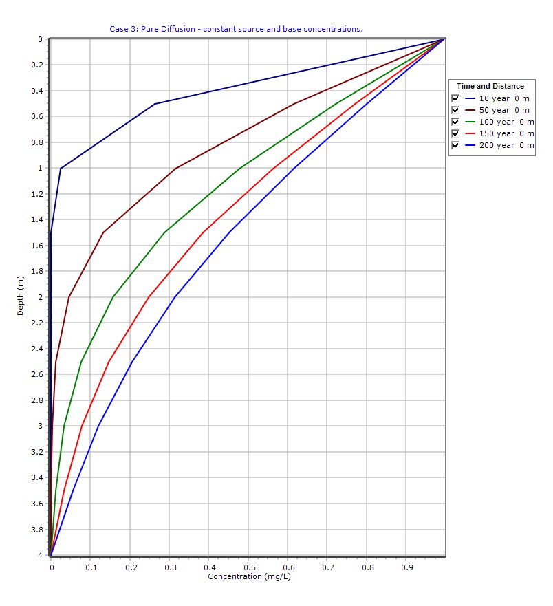
Graphical Output: Depth vs Concentration
PDF Report
 Loading…
Interpretation of Results
1. Development of Concentration Gradient
A smooth gradient forms from the top (high concentration) to the bottom (zero concentration).
2. Time-Dependent Diffusion
- Early time: steep gradients near the source
- Later time: deeper penetration into the layer
3. Steady-State Behavior
Over long periods, the system may approach a steady-state profile, depending on conditions.
4. Role of Aquifer Boundary
The zero-concentration boundary ensures continuous downward flux, preventing accumulation.
Why This Example Matters
Although simple, this case is critical because it:
- Establishes a baseline for diffusion-only transport
- Helps validate model setup and parameters
- Provides insight into mass transfer without flow
- Serves as a comparison for more complex scenarios involving:
- Advection
- Sorption
- Decay
Key Takeaways
- Diffusion is driven solely by concentration gradients
- Boundary conditions strongly control system behavior
- Conservative species simplify analysis by removing reactions
- MIGRATEv10 can isolate individual transport processes effectively
Final Thoughts
MIGRATEv10 Example 3 is a foundational case that highlights the importance of understanding basic transport mechanisms before introducing additional complexity. While real-world systems rarely involve pure diffusion alone, this example provides critical insight into how contaminants behave in low-flow or stagnant environments.
In practice, this type of model is useful for:
- Low-permeability soils
- Barrier systems
- Early-stage conceptual modeling
Learn more about our Contaminant Transport Modeling Solutions
MIGRATE Examples
- MIGRATEv10 Example 1: Modeling a RCRA Subtitle D Landfill with a Composite Liner
- MIGRATEv10 Example 2: Composite Liner System with Primary & Secondary Leachate Collection
- MIGRATEv10 Example 4: Finite Mass Source and Aquifer Mixing with Base Outflow
- MIGRATEv10 Example 5: Understanding Integration, Accuracy, and the Role of Engineering Judgment
- MIGRATEv10 Example 6: Eliminating Negative Concentrations Through Improved Integration
- MIGRATEv10 Example 7: Improving Accuracy with User-Selected Fourier Integration
- MIGRATEv10 Example 8: Evaluating Contaminant Migration at Multiple Lateral Positions
- MIGRATEv10 Example 9: Comparison with the TDAST Analytical Solution
- MIGRATEv10 Example 10: Contaminant Transport in Fractured Media with Sorption
- MIGRATEv10 Example 11: Contaminant Migration from Two Adjacent Landfill Cells
- MIGRATEv10 Example 12: Modeling Time-Dependent Source Histories for Multiple Landfill Cells
- MIGRATEv10 Example 13: Termination of Primary Leachate Collection System
Comparison between POLLUTE and MIGRATE
- MIGRATEv10 vs POLLUTEv10: Pure Diffusion Comparison
- MIGRATEv10 vs POLLUTEv10: Advective–Diffusive Transport Comparison
- MIGRATEv10 vs POLLUTEv10: Finite Mass Source Comparison
- MIGRATEv10 vs POLLUTEv10: Hydraulic Trap (Finite Mass Source) Comparison
- MIGRATEv10 vs POLLUTEv10: Fractured Layer with Sorption Comparison