POLLUTEv10 Example 10: Time-Varying Advective–Dispersive Transport from a Landfill

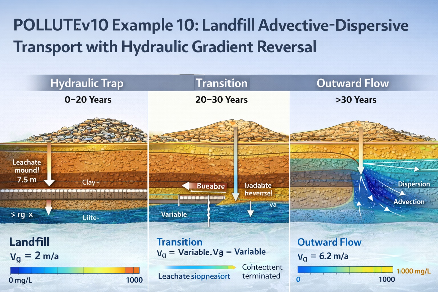
Modeling Hydraulic Gradient Reversal with Variable Properties

POLLUTEv10 Example 10 demonstrates one of the most powerful capabilities of the model: simulating time-varying transport conditions using the Variable Properties feature.

This scenario captures a realistic landfill lifecycle where:

• Early operation creates a hydraulic trap (inward gradient)
• Later conditions cause a gradient reversal
• Contaminant transport shifts from contained → released

---

Problem Overview

This example models:

• A landfill with finite contaminant mass
• A conservative species (no sorption, Kd = 0)
• A leachate collection system that is later discontinued
• A clay liner overlying an aquifer

Key Phases

1. 0–20 years
   • Leachate collection active
   • Inward gradient → hydraulic trap
   • No contaminant escape
2. 20–30 years
   • Collection stops
   • Leachate mound builds
   • Gradient begins to reverse
3. >30 years
   • Outward flow established
   • Contaminant begins migrating into aquifer

---

Conceptual Model

The system includes:

• A 4 m thick clay layer beneath the landfill
• An underlying aquifer
• A finite contaminant source within the landfill
• Time-dependent Darcy velocities (va and vb)

The most critical behavior is the reversal of hydraulic gradient, which fundamentally changes transport direction.

---

Key Equations

Hydrodynamic Dispersion

$D = D_m + \alpha \frac{v_a}{n}$

Where:

• D = hydrodynamic dispersion coefficient
• Dm = molecular diffusion coefficient
• α = dispersivity
• va = Darcy velocity
• n = porosity

Outflow Velocity Relationship

$$v_b = 2 + 200 \cdot v_a$$

• At 30 years, $v_b = 6.2 \, \text{m/a}$

---

Input Parameters

Property	Value	Units
Darcy Velocity (va)	Variable	m/a
Diffusion Coefficient (Dm)	0.02	m²/a
Distribution Coefficient	0.0	cm³/g
Dispersivity (va < 0)	0.0	m
Dispersivity (va > 0)	0.4	m
Soil Porosity (n)	0.4	–
Dry Density	1.5	g/cm³
Soil Thickness	4.0	m
Sub-layers	12	–
Source Concentration	1000	mg/L
Leachate Height (Hr)	7.5	m

Aquifer Properties

Property	Value	Units
Length (L)	200	m
Width (W)	1	m
Thickness (h)	1	m
Porosity (nb)	0.3	–
Outflow Velocity	Variable	m/a

---

Finite Mass Source Calculation

The contaminant mass per unit area:

$$m_{tc} = 0.002 \times 600 \times 6.25 = 7.5 \, \text{kg/m}^2$$

This yields the reference leachate height:

$$H_r = 7.5 \, \text{m}$$

This ensures the model represents a finite, depleting contaminant source.

---

Time-Varying Flow Conditions

Infiltration & Collection

$$Q_c = q_o – v_a = 0.3 – v_a$$Where:

• qo = 0.3 m/a (infiltration through cover)
• va = exfiltration through base

---

Variable Dispersivity Behavior

A key feature of this example:

• va < 0 (inward flow):
  • Dispersivity = 0
  • Transport = diffusion only
• va > 0 (outward flow):
  • Dispersivity = 0.4 m
  • Transport = advection + dispersion

This reflects real-world physics:

• No plume spreading during containment
• Significant plume spreading after release

---

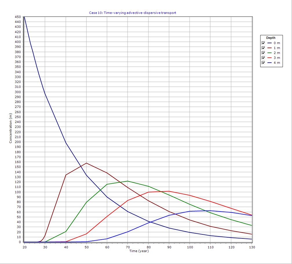
Graphical Output: Concentration vs Time

---

PDF Report

---

Key Insights

• Hydraulic traps are temporary if conditions change
• Leachate collection systems are critical for containment
• Gradient reversal can trigger sudden contaminant release
• Dispersion becomes significant only during outward flow

---

Importance of Sub-Layer Resolution

Accuracy depends on the number of sub-layers when using Variable Properties.

Why?

• Time-dependent parameters require fine numerical resolution
• Velocity reversals create sharp transitions
• Coarse meshes may miss key behaviors

Best Practice

• Use ≥ 12 sub-layers (minimum)
• Increase for sensitivity analysis

---

Practical Applications

This example is highly relevant for:

• Landfill design and risk assessment
• Long-term contaminant migration modeling
• Leachate collection system evaluation
• Regulatory compliance studies

---

Conclusion

POLLUTEv10 Example 10 highlights the complexity of time-dependent transport systems, demonstrating that:

• Flow conditions can change dramatically over time
• Containment strategies must consider future scenarios
• Variable properties modeling is essential for realistic predictions

This example is a powerful tool for understanding how engineering controls and hydrogeology interact to influence contaminant fate.

---