POLLUTEv10 Example 15: Modeling Leachate Collection System Failure Using Variable Properties and Passive Sink

Introduction

POLLUTEv10 Example 15 builds directly on Example 14 by introducing a critical real-world scenario: failure of the primary leachate collection system (LCS). This example demonstrates how to simulate time-dependent changes in hydraulic conditions using the Variable Properties feature in combination with the Passive Sink option.

The result is a more realistic representation of landfill performance over time, particularly as engineered systems degrade.

---

Conceptual Model Overview

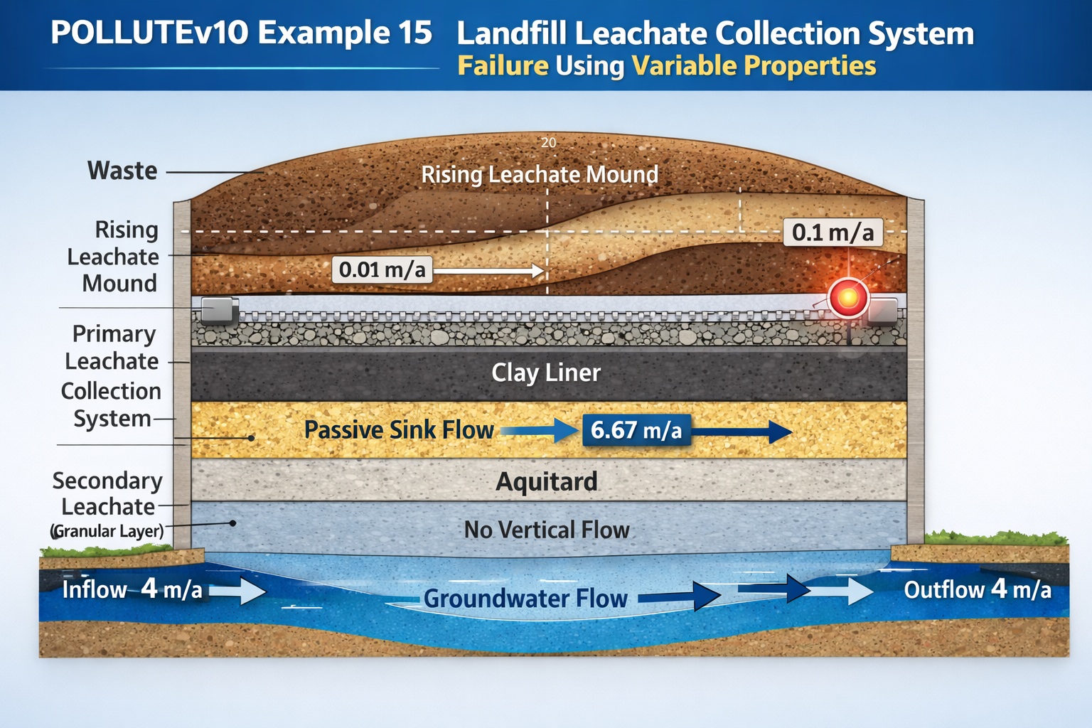
This model represents:

• A landfill with finite contaminant mass
• A failing primary leachate collection system
• A secondary leachate collection system (passive sink)
• An underlying aquifer with fixed outflow

Key Difference from Example 14

• Darcy velocity between landfill and secondary system is time-dependent
• Represents progressive failure of the primary LCS

---

Time-Dependent Hydraulic Behavior

The defining feature of this example is the variation in Darcy velocity (va) over time:

Time Period	Darcy Velocity (va)
0–20 years	0.01 m/a
20–30 years	Linear increase
>30 years	0.1 m/a

Interpretation

• 0–20 years: System functioning normally
• 20–30 years: Gradual failure, leachate mound rises
• After 30 years: Complete failure, increased leakage

This increase in Darcy velocity reflects greater downward migration of contaminants.

---

Source Term and Initial Conditions

As in Example 14:

• Peak concentration: 1000 mg/L
• Reference height of leachate:

$$H_r = 7.5 \, \text{m}$$

• Rate of concentration increase:

$$c_r = 0$$

The contaminant source is finite and conservative, meaning no decay or sorption occurs.

---

Leachate Generation

The water balance equation becomes:$$Q_c = q_0 – v_a = 0.3 – v_a$$

Where:

• $q_0 = 0.3 \, \text{m/a}$ (infiltration)
• $v_a$va​ varies with time

Key Insight

As the primary system fails:

• $v_a$va​ increases
• $Q_c$Qc​ (collected leachate) decreases
• More leachate escapes downward into the subsurface

---

Passive Sink Layer Configuration

The system is divided into three layers:

Layer 1 – Clay Layer

• Variable vertical flow (time-dependent)
• No horizontal flow

Layer 2 – Secondary LCS (Granular Layer)

• Horizontal flow defined as:

$$v_s = \frac{(v_{a2} – v_{a1}) \times 200}{0.3}$$

• Acts as a passive sink, intercepting leachate

Layer 3 – Aquitard

• No advective flow
• Diffusion-dominated transport

---

Coupling Variable Properties and Passive Sink

A critical modeling detail:

• POLLUTE multiplies Darcy velocities from both features
• Recommended approach:
  • Set Darcy velocity = 1.0 in one feature
  • Input actual values in the other

In This Example

• Variable Properties → 1.0
• Passive Sink → actual time-dependent velocities

This avoids unintended scaling errors.

---

Dispersivity Consideration

Using Variable Properties allows inclusion of dispersivity:

• Dispersivity = 0.4 m

This reflects enhanced spreading of contaminants due to outward flow conditions.

---

Model Parameters

Property	Symbol	Value	Units
Darcy Velocity	va	Variable	m/a
Sink Velocity	vs	Variable	m/a
Diffusion Coefficient	D	0.02	m²/a
Dispersivity	α	0.4	m
Distribution Coefficient	Kd	0.0	cm³/g
Soil Porosity	n	0.4	–
Granular Porosity	n	0.3	–
Dry Density	ρd	1.5	g/cm³
Layer Thicknesses	H	1 / 0.3 / 2	m
Source Concentration	c₀	1000	mg/L
Reference Height	Hr	7.5	m
Leachate Collected	Qc	Variable	m/a
Landfill Length	L	200	m
Aquifer Velocity	vb	4	m/a

---

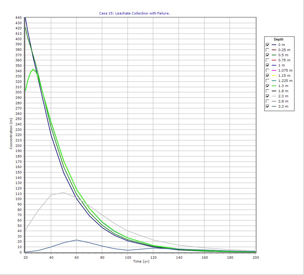
Graphical Output: Concentration vs Time

---

PDF Report

---

---

Key Insights

• System failure dramatically increases contaminant migration risk
• Passive sink helps mitigate but not eliminate impacts
• Time-dependent modeling is essential for:
  • Long-term landfill performance
  • Risk assessment
• Decreasing leachate collection efficiency leads to:
  • Increased downward flux
  • Greater reliance on natural attenuation

---

Numerical Considerations

When using Variable Properties:

• Accuracy depends on number of sublayers
• More sublayers = better resolution of time-dependent changes
• Important for capturing gradual system failure

---

Practical Implications

This example highlights:

• The importance of redundancy in landfill design
• Risks associated with aging infrastructure
• Need for long-term monitoring and maintenance

---

Important Disclaimer

⚠️ This example is hypothetical and intended for demonstration purposes only.

• Not a design guideline
• Not universally applicable
• Requires expert interpretation

These modeling approaches should only be applied by professionals with expertise in:

• Hydrogeology
• Contaminant transport
• Landfill engineering

---

Conclusion

POLLUTEv10 Example 15 provides a powerful demonstration of how system failure can be incorporated into contaminant transport modeling. By combining Variable Properties with the Passive Sink feature, the model captures the dynamic behavior of landfill systems over time—offering valuable insight into long-term environmental risk.