
Introduction
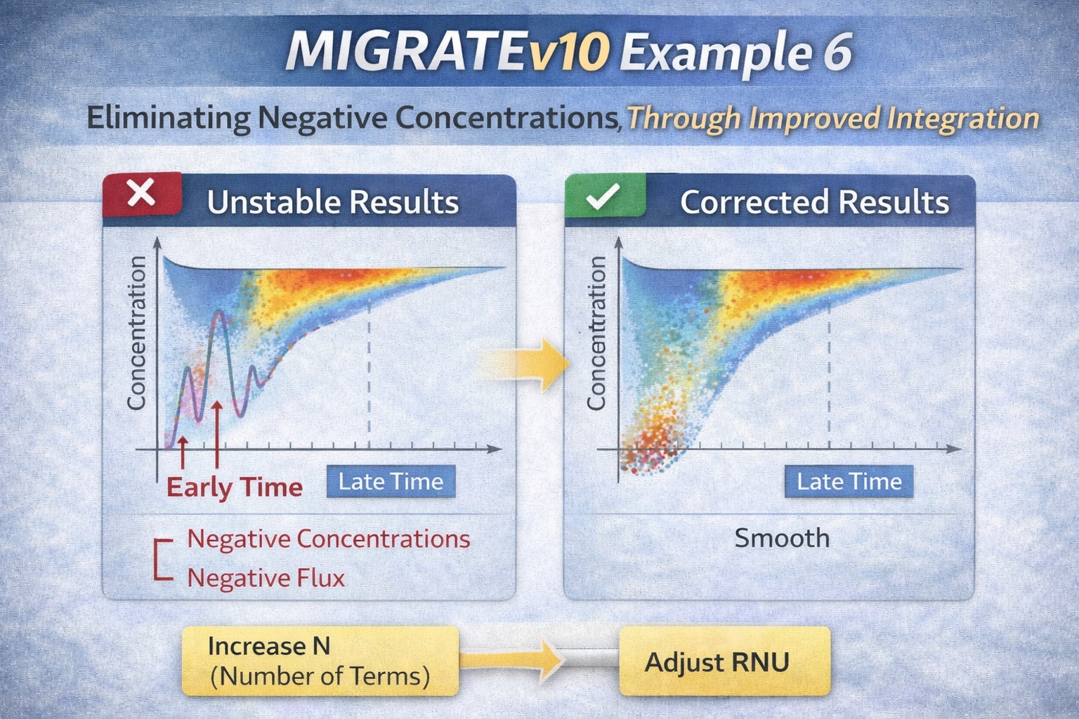
MIGRATEv10 Example 6 builds directly on Example 5 by addressing a common numerical issue in contaminant transport modeling:
👉 Negative concentrations and flux values
These results are non-physical and indicate that numerical integration parameters need adjustment. This example demonstrates how to refine the solution by modifying key Talbot integration parameters, and optionally verifying results using Fourier integration.
Conceptual Overview
This example compares:
- Unstable numerical results (Example 5)
- Refined, stable solutions after adjusting integration parameters
Problem Identified in Example 5
In Example 5, the model output showed:
- ❌ Negative concentrations
- ❌ Negative flux into the base
Why This Happens
These issues arise from:
- Insufficient numerical integration resolution
- Difficulty resolving:
- Very small concentrations
- Early-time or late-time behavior
Key Solution: Adjust Talbot Integration Parameters
The first parameters to examine are:
1. N (Number of Terms)
- Controls the resolution of the numerical inversion
- Higher N → more accurate results
- But also → increased computation time
2. RNU (Scaling Parameter)
- Controls the contour used in Talbot inversion
- Affects stability and convergence of the solution
Important Note
Other Talbot parameters typically do not need adjustment.
👉 Focus first on N and RNU for most cases.
Optional Verification: Fourier Integration
To confirm the accuracy of results, users can:
- Run the same scenario using Fourier integration
Why This Helps
- Provides an independent numerical solution
- Helps verify that results are:
- Stable
- Physically realistic
Modeling Approach in MIGRATEv10
Step 1: Review Output from Example 5
- Identify:
- Negative concentrations
- Negative flux values
Step 2: Increase Talbot Parameter N
- Gradually increase number of terms
- Observe effect on solution stability
Step 3: Adjust RNU if Needed
- Fine-tune scaling for improved convergence
Step 4: Re-run Simulation
- Check if:
- Oscillations are removed
- Results are physically realistic
Step 5: Optional Cross-Check
- Run using Fourier integration
- Compare results
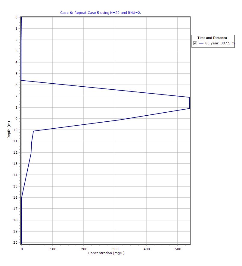
Graphical Output: Depth vs Concentration
PDF Report
 Loading…
Interpretation of Results
Before Adjustment
- Oscillating concentration curves
- Negative values (non-physical)
- Unstable flux calculations
After Adjustment
- Smooth concentration profiles
- Physically realistic values
- Stable flux behavior
When to Increase Integration Parameters
You should refine integration when:
- Results show non-physical behavior
- Concentrations are very small
- Simulation is:
- Far before peak concentration
- Far after peak concentration
Trade-Off: Accuracy vs Computation Time
| Parameter Increase | Effect |
|---|---|
| Higher N | More accurate, slower |
| Adjusted RNU | More stable solution |
| Fourier check | More confidence, extra runtime |
👉 The goal is to find a balance between accuracy and efficiency
Key Takeaways
- Negative concentrations are a numerical issue—not a physical result
- N and RNU are the primary parameters for fixing instability
- Most cases do not require adjusting all Talbot parameters
- Fourier integration is useful for validation
- Always verify results with engineering judgment
Practical Tips
- Start with moderate increases in N
- Avoid excessive computation unless needed
- Use parametric testing when results are uncertain
- Always inspect output files carefully
Final Thoughts
MIGRATEv10 Example 6 reinforces a critical lesson:
Accurate modeling requires both numerical understanding and engineering judgment
By refining integration parameters, users can eliminate non-physical results and ensure that model outputs are both:
- Numerically stable
- Physically meaningful
This example is essential for anyone performing high-precision contaminant transport modeling, especially when working with:
- Low concentrations
- Long simulation times
- Sensitive boundary conditions
Learn more about our Contaminant Transport Modeling Solutions
MIGRATE Examples
- MIGRATEv10 Example 1: Modeling a RCRA Subtitle D Landfill with a Composite Liner
- MIGRATEv10 Example 2: Composite Liner System with Primary & Secondary Leachate Collection
- MIGRATEv10 Example 3: Pure Diffusion of a Conservative Contaminant
- MIGRATEv10 Example 4: Finite Mass Source and Aquifer Mixing with Base Outflow
- MIGRATEv10 Example 5: Understanding Integration, Accuracy, and the Role of Engineering Judgment
- MIGRATEv10 Example 7: Improving Accuracy with User-Selected Fourier Integration
- MIGRATEv10 Example 8: Evaluating Contaminant Migration at Multiple Lateral Positions
- MIGRATEv10 Example 9: Comparison with the TDAST Analytical Solution
- MIGRATEv10 Example 10: Contaminant Transport in Fractured Media with Sorption
- MIGRATEv10 Example 11: Contaminant Migration from Two Adjacent Landfill Cells
- MIGRATEv10 Example 12: Modeling Time-Dependent Source Histories for Multiple Landfill Cells
- MIGRATEv10 Example 13: Termination of Primary Leachate Collection System
Comparison between POLLUTE and MIGRATE
- MIGRATEv10 vs POLLUTEv10: Pure Diffusion Comparison
- MIGRATEv10 vs POLLUTEv10: Advective–Diffusive Transport Comparison
- MIGRATEv10 vs POLLUTEv10: Finite Mass Source Comparison
- MIGRATEv10 vs POLLUTEv10: Hydraulic Trap (Finite Mass Source) Comparison
- MIGRATEv10 vs POLLUTEv10: Fractured Layer with Sorption Comparison